Section 9: LATENT DIRICHLET ALLOCATION
Pratheepa Jeganathan
04 August, 2021
09_latent_Dirichlet_allocation.Rmd
library(phyloseq)
library(tidyverse)
library(genefilter)
library(Rcpp)
library(rstan)
library(randomcoloR)
library(DESeq2)
library(diffTop)
theme_set(theme_minimal())
theme_update(
  text = element_text(size = 10),
  legend.text = element_text(size = 10)
)
Here, we are interested infer on the topics (bacterial communities) when we use original and modified PNA clams (two different experimental conditions). We use latent Dirichlet allocation to identify topics.
Data
In this workflow we use psE_BARBI phyloseq object in this package. In psE_BARBI, we removed DNA contaminants using BARBI.
Preprocessing
We choose ASVs that have at least 25 counts in at least two specimens.
threshold <- kOverA(2, A = 25)
ps <- phyloseq::filter_taxa(
  ps,
  threshold, TRUE)
## Found more than one class "phylo" in cache; using the first, from namespace 'phyloseq'## Also defined by 'tidytree'
ps## phyloseq-class experiment-level object
## otu_table() OTU Table: [ 1418 taxa and 86 samples ]
## sample_data() Sample Data: [ 86 samples by 16 sample variables ]
## tax_table() Taxonomy Table: [ 1418 taxa by 6 taxonomic ranks ]
## phy_tree() Phylogenetic Tree: [ 1418 tips and 1417 internal nodes ]
ps <- prune_taxa(taxa_sums(ps) > 0, ps)## Found more than one class "phylo" in cache; using the first, from namespace 'phyloseq'
## Also defined by 'tidytree'
ps## phyloseq-class experiment-level object
## otu_table() OTU Table: [ 1418 taxa and 86 samples ]
## sample_data() Sample Data: [ 86 samples by 16 sample variables ]
## tax_table() Taxonomy Table: [ 1418 taxa by 6 taxonomic ranks ]
## phy_tree() Phylogenetic Tree: [ 1418 tips and 1417 internal nodes ]Edit specimen names
We edit specimen names and identify Asteraceae and non-Asteraceae plants.
sam_names <- str_replace(sample_names(ps), "E106", "E-106")
sam_names <- str_replace(sam_names, "_F_filt.fastq.gz", "")
sam_names <- str_replace(sam_names, "Connor-", "E")
sample_names(ps) <- sam_names
sample_data(ps)$X <- sam_names
sample_data(ps)$unique_names <- sam_names
aster <- c("142","143","15","ST","22","40")
non_aster <- c("33", "71", "106")

paired_aster <- c("E-142-1", "E142-1", "E-142-5", "E142-5", "E-142-10", "E142-10", "E-143-2", "E143-2", "E-143-7", "E143-7", "E-15-1", "E15-1", "ST-CAZ-4-R-O", "ST-CAZ-4-R-M", "ST-SAL-22-R-O", "ST-SAL-22-R-M", "ST-TRI-10-R-O", "ST-TRI-10-R-M")
paired_non_aster <- c("E33-7", "E-33-7", "E33-8", "E-33-8", "E33-9", "E-33-9", "E71-10", "E-71-10","E71-2","E-71-2" ,"E71-3", "E-71-3", "E106-1", "E-106-1", "E106-3", "E-106-3", "E106-4", "E-106-4")
paired_specimens <- c(paired_aster, paired_non_aster)
Choose colors for plots. We will use nine colors for nine different plants in the dataset.
plant_colors <- c("#999999", "#E69F00", "#56B4E9", "#009E73", "#F0E442", "#0072B2", "#D55E00", "#CC79A7", "purple")Input data for LDA
Based on the ordination, we choose the number of topics as K=11. We set the hyperparameters \(\alpha = 0.8\) and \(\gamma = 0.8\).
K <- 11
alpha <- 0.8
gamma <- 0.8
stan.data <- setUpData(
  ps = ps,
  K = K,
  alpha = alpha,
  gamma = gamma
)
Posterior sampling
We need to estimate \(\theta\) and \(B = \left[\beta_{1}, \cdots, \beta_{K} \right]^{T}.\)
We estimate the parameters using HMC NUTS with four chains and 2000 iterations. Out of these 2000 iterations, 1000 iterations were used as warm-up samples.
We use high-performance computing and save the results.
We specify a file name.
fileN <- paste0(
  "JABES_Endo_all_K_",
  K,
  "_ite_",
  iter,
  ".RData"
  )
iter <- 2000
chains <- 4

stan.fit <- LDAtopicmodel(
  stan_data = stan.data,
  iter = iter,
  chains = chains,
  sample_file = NULL,
  diagnostic_file = NULL,
  cores = 4,
  control = list(adapt_delta = 0.9),
  save_dso = TRUE,
  algorithm = "NUTS"
  )
save(stan.fit, file = fileN)
We extract posterior samples from the results.
samples <- rstan::extract(
  stan.fit,
  permuted = TRUE,
  inc_warmup = FALSE,
  include = TRUE
  )
Alignment
We estimated the parameters using the HMC-NUTS sampler with four chains and 2000 iterations. Out of these 2000 iterations, 1000 iterations were used as warm-up samples and discarded. Label switching across chains makes it difficult to directly compute log predictive density, split-\(\hat{R}\), effective sample size for model assessment, and evaluate convergence and mixing of chains.
To address this issue, we fixed the order of topics in chain one and then found the permutation that best aligned the topics across all four chains. For each chain two to four, we identified the estimated topics pair with the highest correlation, then found the next highest pair among the remaining, and so forth.
We create a Topic \(*\) Chain matrix.
theta <- samples$theta

aligned <- alignmentMatrix(
  theta,
  ps,
  K,
  iterUse = iter/2,
  chain = chains,
  SampleID_name = "unique_names"
  )
Align topic proportion
We align the topic proportion in each specimen across four chains.
theta_aligned <- thetaAligned(
  theta,
  K,
  aligned,
  iterUse = iter/2,
  chain = chains
  )
Align ASV proportion
We align the ASVs proportion in each topic across four chains.
beta <- samples$beta


beta_aligned <- betaAligned(
  beta,
  K,
  aligned,
  iterUse = iter/2,
  chain = chains
  )
Visualization
Plot topic proportion
Plot the topic proportion in specimens and we can save it for publication purposes. We can draw an informative summary of bacterial communities in each phenotype.
p <- plotTopicProportion(
  ps,
  theta_aligned,
  K,
  col_names_theta_all = c("iteration", "Sample", "Topic", "topic.dis"),
  chain = 4,
  iterUse = iter/2,
  SampleIDVarInphyloseq = "unique_names",
  design = ~ pna
)

ggsave(paste0("topic_dis_all_",K, ".png")), p, width = 30, height = 16)
Figure 6: Topic distribution in specimens from Sonchus Arvensis plant. The color gradient represents the median topic distribution.
Plot ASVs distribution
We plot the ASVs distribution in each topic.
p <- plotASVCircular(
  ps,
  K,
  iterUse = iter/2,
  chain = chains,
  beta_aligned,
  varnames = c("iterations", "topic", "rsv_ix"),
  value_name = "beta_h",
  taxonomylevel = "Class",
  thresholdASVprop = 0.008
  )

ggsave(paste0("circular_plot_plant_all_K_", K, ".png"), p, width = 28, height = 22)
Figure 7: ASV distribution over topics in all specimens
Model assessement
We do goodness of fit test using the posterior estimates and observed data.
p_hist <- modelAssessment(
  ps,
  stan.fit,
  iterUse = iter/2,
  statistic = "max",
  ASVsIndexToPlot = c(1, 3, 10:14, 19:26, 36, 51:53, 148)
)

ggsave(
  paste0(
    "model_assesment_hist_all_obs_sim_K_",
    K,
    ".png"
    ),
  p_hist,
  width = 12,
  height = 6
  )
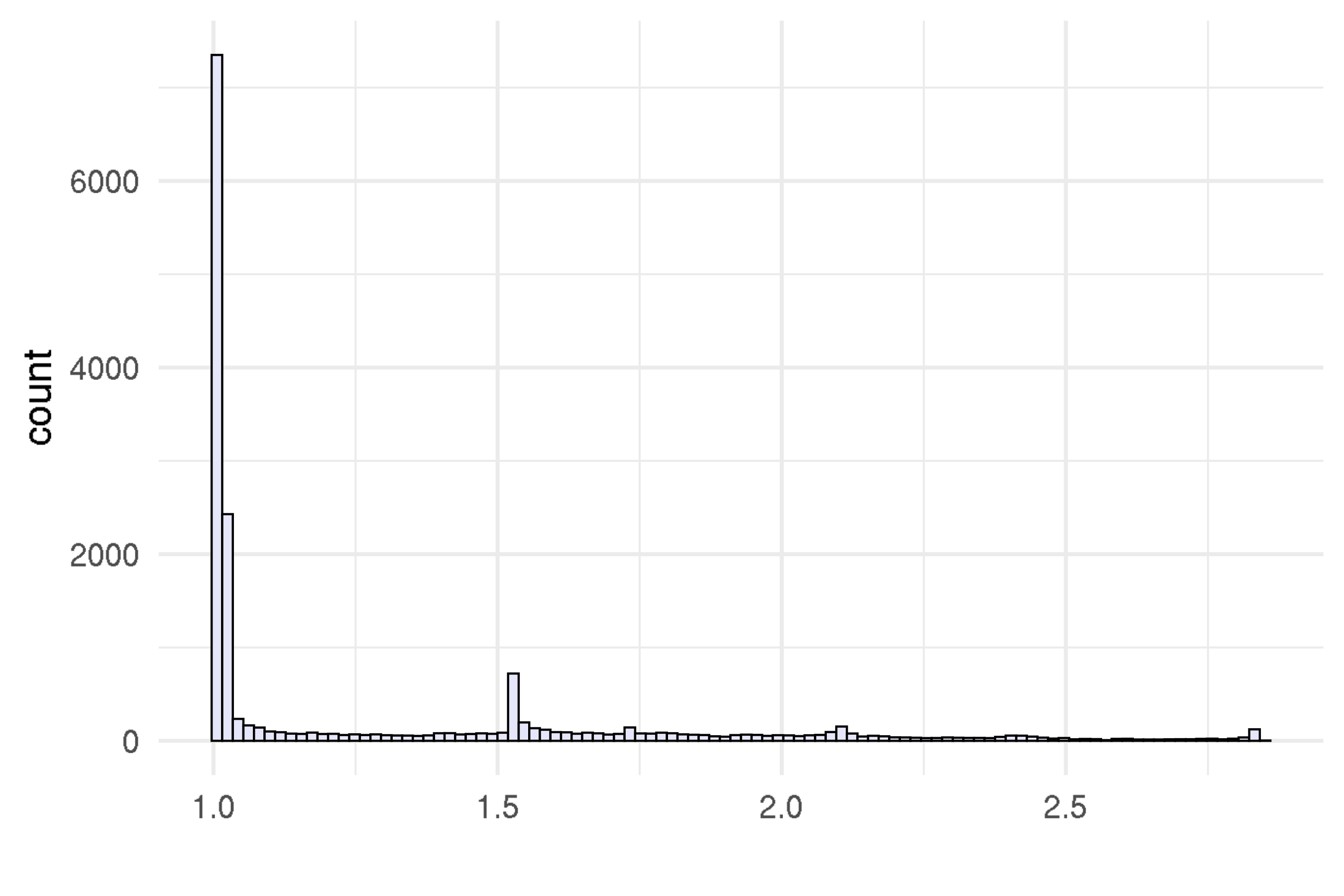
Supplementary Figure 13: Predictive model check with simulated data, observed data, and a statistic G(Kij) = max{Kij}. Each facet shows the histogram of G(Kij) of each ASV in specimens from the posterior predictive distribution and the vertical line shows the value of G (Kij ) of each ASV in observed data.
Diagnostics
Effective sample size (ESS)
We compute effective sample size for each parameter.
p <- diagnosticsPlot(
  theta_aligned = theta_aligned,
  beta_aligned = beta_aligned,
  iterUse = iter/2,
  chain = 4
)
p_ess_bulk <- p[[[1]]]

ggsave(
  paste0("ess_bulk_plant_all_K_", K, ".png"),
  p_ess_bulk,
  width = 9,
  height = 6
  )
Supplementary Figure 14: Effective sample size (ESS) with eleven topics.
\(\hat{R}\)
We can check whether \(\hat{R}\) is less than 1.02.
p_rhat <- p[[2]]

ggsave(
  paste0("Rhat_plant_all_K_", K, ".png"),
  p_rhat,
  width = 9,
  height = 6
  )
Supplementary Figure 15: Split Rhat with eleven topics.
Differential topic analysis
Test on all specimens
We do test on all specimens. We can write DESeq2 results to LaTex.
dds_all <- diffTopAnalysis(
  design = ~ pna,
  ps,
  theta_aligned,
  subsetSample = sample_names(ps),
  fitType = "mean"
)

saveRDS(
  dds_all,
  file = paste0("dds_all_K_", K,".rds")
)## log2 fold change (MLE): pna O vs M
## Wald test p-value: pna O vs M
## DataFrame with 11 rows and 6 columns
## baseMean log2FoldChange lfcSE stat pvalue padj
## <numeric> <numeric> <numeric> <numeric> <numeric> <numeric>
## Topic_1 12980.2689 -0.902957 0.954118 -0.946379 3.43955e-01 0.609485512
## Topic_2 1388.4912 0.328641 0.691155 0.475495 6.34434e-01 0.719579869
## Topic_3 14.5487 -0.559488 0.584374 -0.957414 3.38358e-01 0.609485512
## Topic_4 6138.5557 2.056851 0.749974 2.742564 6.09615e-03 0.022352555
## Topic_5 50.1848 2.693638 0.665150 4.049672 5.12894e-05 0.000564184
## Topic_6 5002.9019 -0.285674 0.795705 -0.359020 7.19580e-01 0.719579869
## Topic_7 25.1418 -0.382548 0.498956 -0.766696 4.43262e-01 0.609485512
## Topic_8 642.9452 0.638403 0.749673 0.851575 3.94450e-01 0.609485512
## Topic_9 728.3070 0.780513 0.781941 0.998174 3.18195e-01 0.609485512
## Topic_10 2452.9197 2.617431 0.725300 3.608757 3.07668e-04 0.001692175
## Topic_11 6788.9347 0.330308 0.782177 0.422294 6.72811e-01 0.719579869
#writeResTable(res, fileN = paste0("dds_all_K_", K,".tex"))Test on paired-specimens
We do the test on paired-specimens.
dds_all_paired <- diffTopAnalysis(
  design = ~ pna,
  ps,
  theta_aligned,
  subsetSample = paired_specimens
)

saveRDS(
  dds_all_paired,
  file = paste0("dds_all_paired_K_", K,".rds")
)## log2 fold change (MLE): pna O vs M
## Wald test p-value: pna O vs M
## DataFrame with 11 rows and 6 columns
## baseMean log2FoldChange lfcSE stat pvalue padj
## <numeric> <numeric> <numeric> <numeric> <numeric> <numeric>
## Topic_1 3983.7697 -9.412600 1.056278 -8.911103 5.05275e-19 5.55802e-18
## Topic_2 898.6700 1.491941 0.999725 1.492352 1.35607e-01 2.13097e-01
## Topic_3 23.5763 0.282751 0.924598 0.305810 7.59749e-01 8.12226e-01
## Topic_4 1138.7952 3.371133 0.995722 3.385618 7.10182e-04 1.95300e-03
## Topic_5 31.7514 2.290040 0.892339 2.566333 1.02780e-02 1.88430e-02
## Topic_6 83.5973 0.351490 0.912658 0.385128 7.00143e-01 8.12226e-01
## Topic_7 35.3625 0.233201 0.801434 0.290979 7.71067e-01 8.12226e-01
## Topic_8 393.8606 -0.265216 1.116438 -0.237556 8.12226e-01 8.12226e-01
## Topic_9 468.2304 -6.004885 0.944671 -6.356589 2.06282e-10 7.56369e-10
## Topic_10 1938.0794 3.029427 1.085621 2.790502 5.26263e-03 1.15778e-02
## Topic_11 419.7516 6.324962 0.940052 6.728314 1.71641e-11 9.44024e-11
#writeResTable(res, fileN = paste0("dds_all_paired_K_", K,".tex"))Test on paired non-Aster specimens
We do the test on paired non-Aster specimens.
dds_all_paired_nonaster <- diffTopAnalysis(
  design = ~ pna,
  ps,
  theta_aligned,
  subsetSample = paired_non_aster
)


saveRDS(dds_all_paired_nonaster,
        file = paste0("dds_all_paired_nonaster_K_", K,".rds")
)## log2 fold change (MLE): pna O vs M
## Wald test p-value: pna O vs M
## DataFrame with 11 rows and 6 columns
## baseMean log2FoldChange lfcSE stat pvalue padj
## <numeric> <numeric> <numeric> <numeric> <numeric> <numeric>
## Topic_1 860.20984 -0.00301489 1.571767 -0.00191815 0.998469536 0.99846954
## Topic_2 1040.00766 -0.23883154 1.489550 -0.16033804 0.872614794 0.99846954
## Topic_3 4.72578 -1.96488007 1.042164 -1.88538517 0.059377854 0.16328910
## Topic_4 180.11478 4.32606625 1.204541 3.59146455 0.000328825 0.00361707
## Topic_5 27.56455 2.23657681 1.180879 1.89399299 0.058225941 0.16328910
## Topic_6 6.67586 0.09843585 0.881377 0.11168412 0.911073873 0.99846954
## Topic_7 5.19734 -0.59432231 0.892778 -0.66569966 0.505603089 0.79451914
## Topic_8 425.39352 0.63277929 1.509760 0.41912576 0.675124224 0.92829581
## Topic_9 2991.31585 -2.69366584 1.665720 -1.61711797 0.105852819 0.19406350
## Topic_10 1417.10667 2.41994794 1.495368 1.61829572 0.105598883 0.19406350
## Topic_11 33.61182 3.26394880 1.158670 2.81697937 0.004847764 0.02666270
#writeResTable(res, fileN = paste0("dds_all_paired_nonaster_", K,".tex"))Test on paired Aster specimens
We do the test on paired Aster specimens.
dds_all_paired_aster <- diffTopAnalysis(
  design = ~ pna,
  ps,
  theta_aligned,
  subsetSample = paired_aster
)


saveRDS(
  dds_all_paired_aster,
  file = paste0("dds_all_paired_aster_K_", K,".rds")
)## log2 fold change (MLE): pna O vs M
## Wald test p-value: pna O vs M
## DataFrame with 11 rows and 6 columns
## baseMean log2FoldChange lfcSE stat pvalue padj
## <numeric> <numeric> <numeric> <numeric> <numeric> <numeric>
## Topic_1 6218.5368 -10.4304467 1.51290 -6.8943421 5.41147e-12 5.95261e-11
## Topic_2 808.8041 1.2913524 1.35518 0.9529025 3.40639e-01 6.24506e-01
## Topic_3 62.3447 0.5769415 1.41106 0.4088702 6.82635e-01 8.34332e-01
## Topic_4 3197.9976 0.9723636 1.53691 0.6326749 5.26946e-01 8.28058e-01
## Topic_5 10.5337 -0.1502755 1.27513 -0.1178511 9.06186e-01 9.48164e-01
## Topic_6 188.5282 0.0862107 1.32605 0.0650131 9.48164e-01 9.48164e-01
## Topic_7 20.2758 0.4522516 1.03245 0.4380355 6.61361e-01 8.34332e-01
## Topic_8 12.0123 -1.3189221 1.02924 -1.2814486 2.00036e-01 4.52427e-01
## Topic_9 1035.0590 -7.8134758 1.32604 -5.8923438 3.80756e-09 1.39610e-08
## Topic_10 129.1210 -1.5272929 1.20675 -1.2656214 2.05649e-01 4.52427e-01
## Topic_11 2344.2823 8.3837719 1.38843 6.0383030 1.55743e-09 8.56589e-09
#writeResTable(res, fileN = paste0("dds_all_paired_aster_", K,".tex"))