Section 5: TRANSFORMATIONS

library(phyloseq)
library(tidyverse)
library(genefilter) #KOverA
library(DESeq2)
library(vsn)
library(ade4) # dudi.pca
library(ggrepel) # geom_text_repel
library(hexbin) # for stat_binhex()
devtools::load_all()

theme_set(theme_minimal())
theme_update(
  text = element_text(size = 10),
  legend.text = element_text(size = 10)
)

Data

data("psE_BARBI")
threshold <- kOverA(2, A = 25) 
psE_BARBI <- phyloseq::filter_taxa(psE_BARBI, threshold, TRUE) 
psE_BARBI

## phyloseq-class experiment-level object
## otu_table()   OTU Table:         [ 1418 taxa and 86 samples ]
## sample_data() Sample Data:       [ 86 samples by 16 sample variables ]
## tax_table()   Taxonomy Table:    [ 1418 taxa by 6 taxonomic ranks ]
## phy_tree()    Phylogenetic Tree: [ 1418 tips and 1417 internal nodes ]

ps <- psE_BARBI
rm(psE_BARBI)
ps <- prune_taxa(taxa_sums(ps) > 0, ps)
ps

## phyloseq-class experiment-level object
## otu_table()   OTU Table:         [ 1418 taxa and 86 samples ]
## sample_data() Sample Data:       [ 86 samples by 16 sample variables ]
## tax_table()   Taxonomy Table:    [ 1418 taxa by 6 taxonomic ranks ]
## phy_tree()    Phylogenetic Tree: [ 1418 tips and 1417 internal nodes ]

Edit specimen names

We edit specimen names and identify Asteraceae and non-Asteraceae plants.

sam_names <- str_replace(sample_names(ps), "E106", "E-106")
sam_names <- str_replace(sam_names, "_F_filt.fastq.gz", "")
sam_names <- str_replace(sam_names, "Connor-", "E")
sample_names(ps) <- sam_names
sample_data(ps)$X <- sam_names
sample_data(ps)$unique_names <- sam_names
aster <- c("142","143","15","ST","22","40")
non_aster <- c("33", "71", "106")

paired_aster <- c("E-142-1", "E142-1", "E-142-5", "E142-5", "E-142-10", "E142-10", "E-143-2", "E143-2", "E-143-7", "E143-7", "E-15-1", "E15-1", "ST-CAZ-4-R-O", "ST-CAZ-4-R-M", "ST-SAL-22-R-O", "ST-SAL-22-R-M", "ST-TRI-10-R-O", "ST-TRI-10-R-M")
paired_non_aster <- c("E33-7", "E-33-7", "E33-8", "E-33-8", "E33-9", "E-33-9", "E71-10", "E-71-10","E71-2","E-71-2" ,"E71-3", "E-71-3", "E106-1", "E-106-1", "E106-3", "E-106-3", "E106-4", "E-106-4")
paired_specimens <- c(paired_aster, paired_non_aster)

5.1 Variance stabilization

This workflow is for visualization of 16S rRNA sequencing data. We use 16S after removing contaminants psE_BARBI. Then, we remove ASVs that have at least 25 reads in five specimens. This data set has 1418 ASVs and 86 samples.

Anscombe’s transformation

The following transformation may take long time so we saved it as ps_ans. We can access it from diffTop package.

ps_ans <- phyloseqTransformation(ps  = ps, c = 0.4)

DESeq2 transformation

There are three different transformations in DESEq2 package.

We refer to the help page of varianceStabilizingTransformation() for fitType="mean", fitType="parametric", fitType="local".

phyloseqTransformationVST <- function(
  ps, 
  fitType = "mean"
  ){
      dds <- phyloseq_to_deseq2(
        ps, 
        design = ~ 1
        )
      dds <-  estimateSizeFactors(
        dds, 
        type = "poscounts"
        )
      
      vsd <- varianceStabilizingTransformation(
        dds, 
        blind = FALSE, 
        fitType = fitType
        )
      
      abund_temp <- assay(vsd)
      
      ps <- phyloseq(
        otu_table(abund_temp, taxa_are_rows = TRUE),
        sample_data(ps), 
        tax_table(ps), 
        phy_tree(ps)
        )
      return(ps)
} 

ps_ans_deseq2 <- phyloseqTransformationVST(
  ps, 
  fitType = "mean"
  )
ps_parametric_deseq2 <- phyloseqTransformationVST(
  ps, 
  fitType = "parametric"
  )
ps_local_deseq2 <- phyloseqTransformationVST(
  ps, 
  fitType = "local"
  )

MSD (mean-standard deviation) plots after each transformation

We use meanSdPlot() in vsn package.

data("ps_ans")
msd_ps_ans <- meanSdPlot(
  otu_table(ps_ans) %>% 
    as.matrix(), 
  plot = FALSE)

msd_ps_ans$gg +
  ggtitle("Anscombe's Transformation") +
  theme(plot.title = element_text(hjust = 0.5))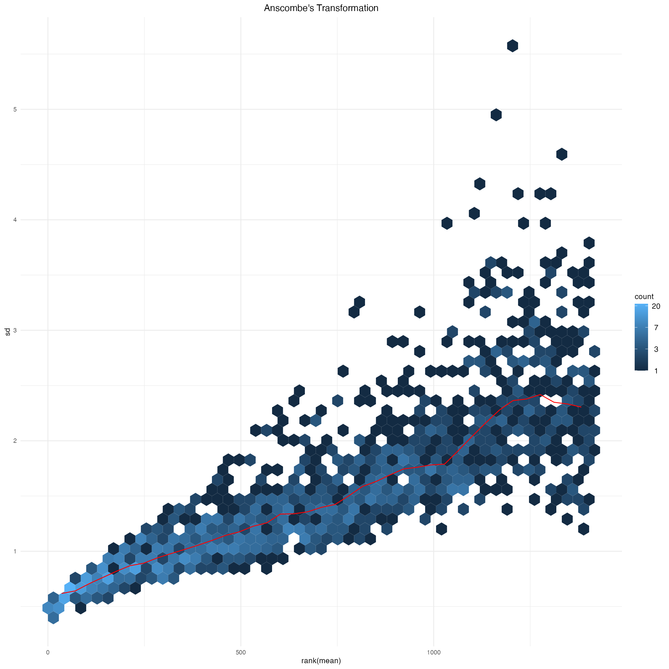

Supplementary Figure 2: Anscombe’s transformation of abundance data.

msd_ps_ans_deseq2 <- meanSdPlot(
  otu_table(ps_ans_deseq2) %>%
    as.matrix(),
  plot = FALSE)

msd_ps_ans_deseq2$gg +
  ggtitle("Anscombe Transformation in DESeq2") +
  theme(plot.title = element_text(hjust = 0.5))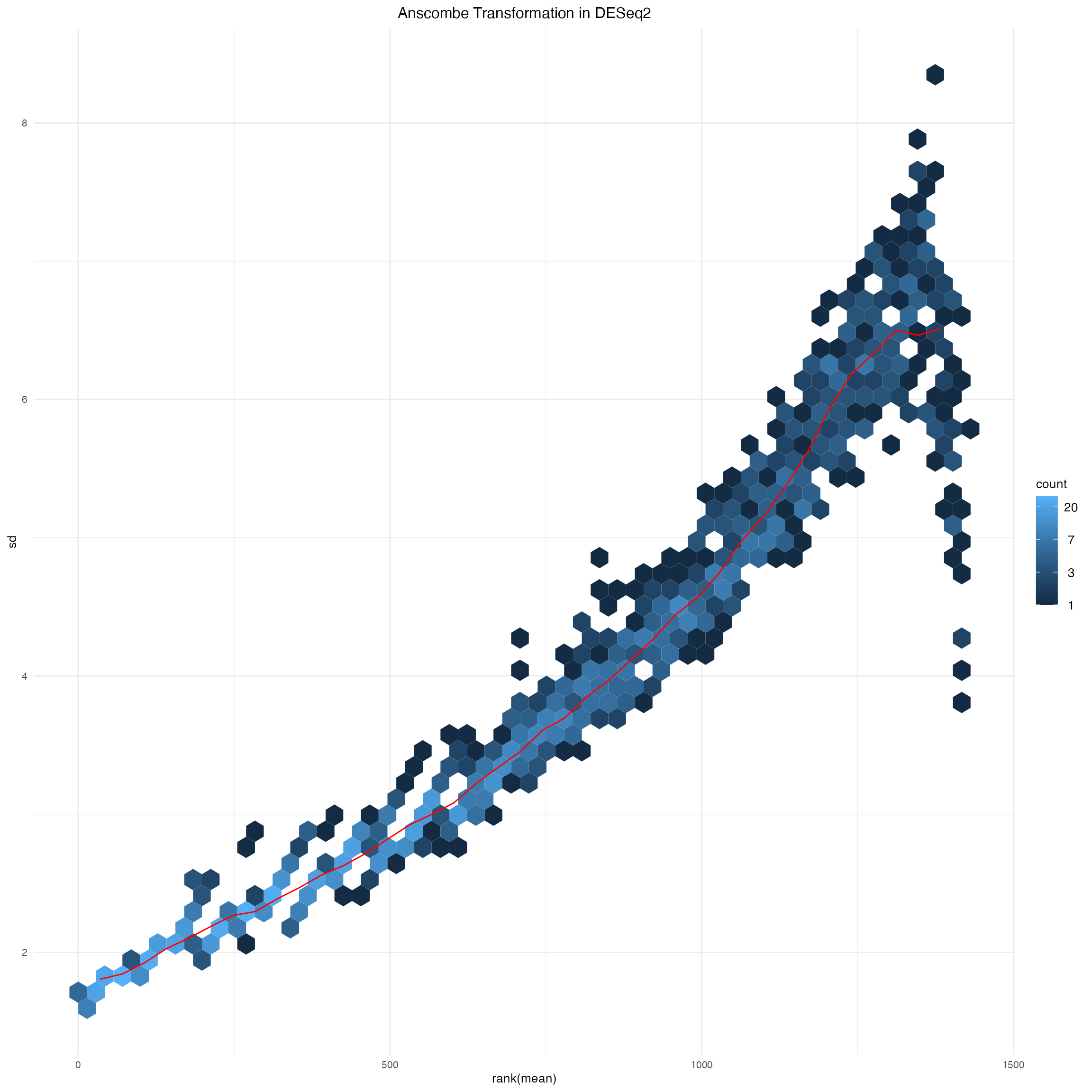

Supplementary Figure 3: Anscombe’s transformation implemented in DESeq2 package.

msd_ps_parametric_deseq2 <- meanSdPlot(
  otu_table(ps_parametric_deseq2) %>%
    as.matrix(),
  plot = FALSE)

msd_ps_parametric_deseq2$gg +
  ggtitle("Parametric Transformation in DESeq2") +
  theme(plot.title = element_text(hjust = 0.5))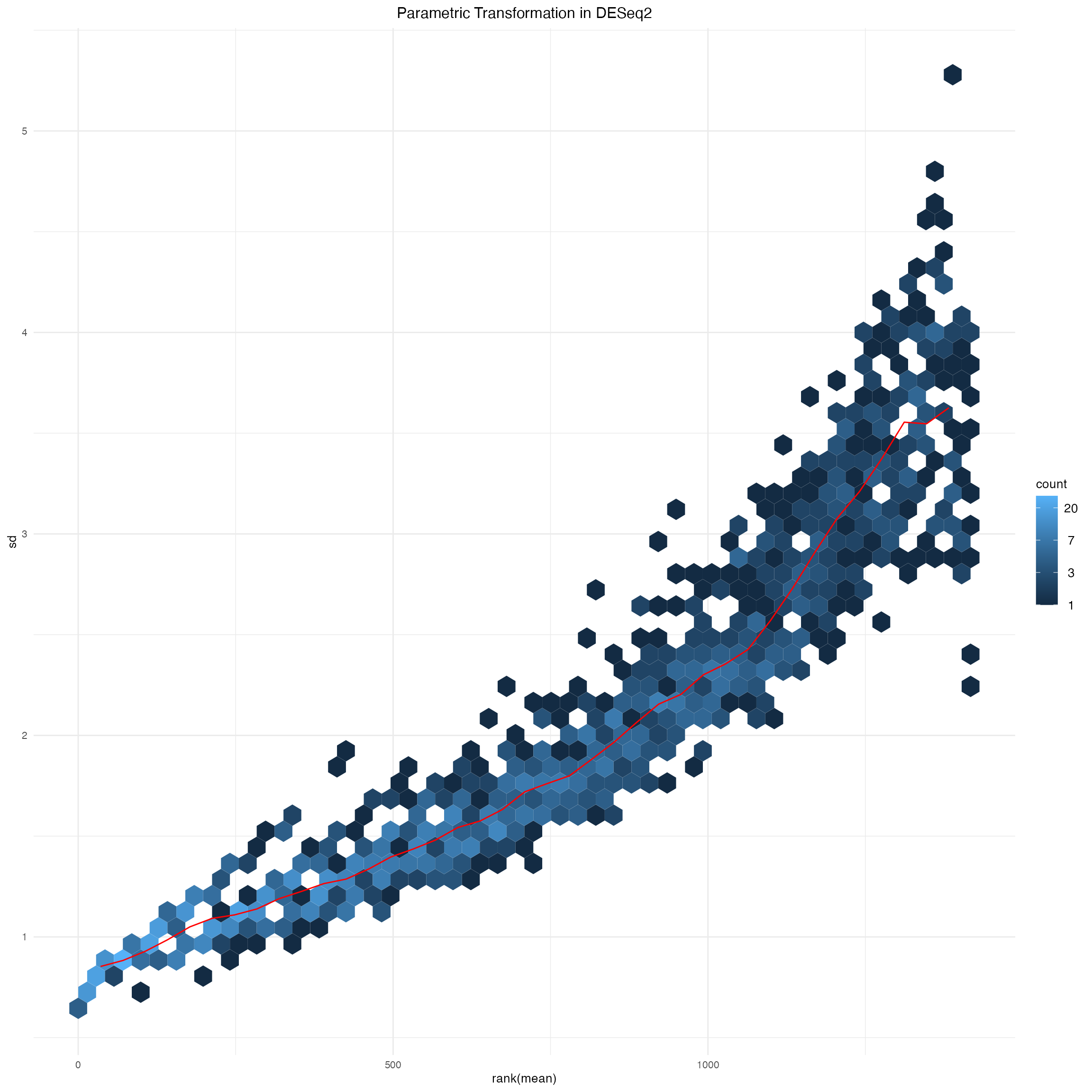

Supplementary Figure 4: Parametric transformation implemented in DESeq2 package.

msd_ps_local_deseq2 <- meanSdPlot(
  otu_table(ps_local_deseq2) %>% 
    as.matrix(),
  plot = FALSE)

msd_ps_local_deseq2$gg +
  ggtitle("Local Transformation in DESeq2") +
  theme(plot.title = element_text(hjust = 0.5))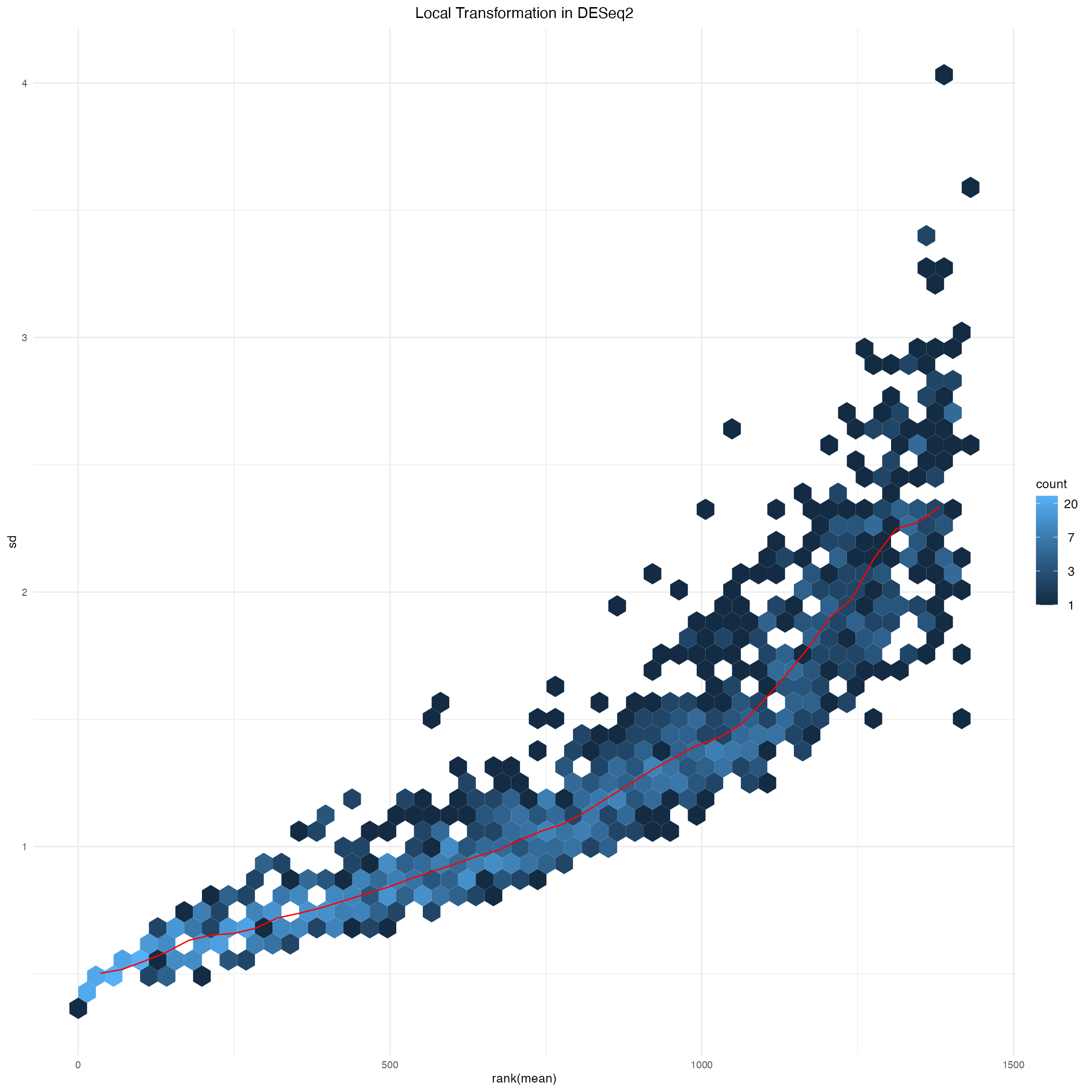

Supplementary Figure 5: Nonparametric transformation implemented in DESeq2 package.

5.2 Rank-based methods

Rank-based transformation

The association between abundances and threshholded ranks, for a few randomly selected samples.

The numbers of the y-axis are those supplied to PCA.

abund <- otu_table(ps_ans) 
abund_ranks <- apply(abund, 2, rank) 
abund_ranks <- abund_ranks - 900
abund_ranks[abund_ranks < 1] <- 1

abund_df <- reshape2::melt(
  abund, 
  value.name = "abund"
  ) %>%
  left_join(
    reshape2::melt(
      abund_ranks, 
      value.name = "rank")
    )


colnames(abund_df) <- c("seq", "sample", "abund",  "rank")

sample_ix <- sample(1:nrow(abund_df), 5)

abund_df_subset <- abund_df %>%
          filter(sample %in% abund_df$sample[sample_ix])

ggplot(abund_df_subset) +
  geom_point(aes(x = abund, y = rank, col = sample),
             position = position_jitter(width = 0.2), 
             size = 2) +
  labs(x = "Abundance", 
       y = "Thresholded rank") +
  scale_color_brewer(palette = "Set2")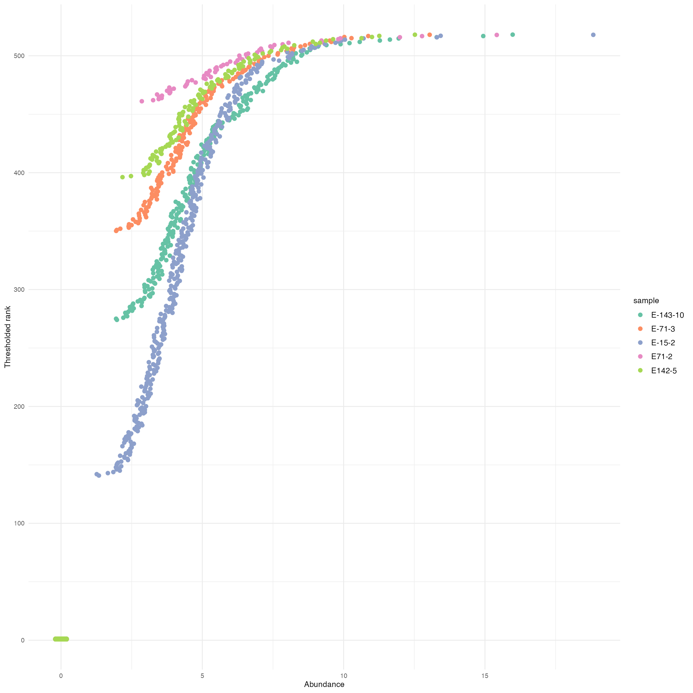

Threshold ranks PCA

# We will use 9 colors for 9 different plants
plant_colors <- c("#999999", "#E69F00", "#56B4E9", "#009E73", "#F0E442", "#0072B2", "#D55E00", "#CC79A7", "purple")

abund_ranks <- t(abund_ranks)

ranks_pca <- dudi.pca(
  abund_ranks, 
  scannf = FALSE, 
  nf = 3)

row_scores <- data.frame(
  li = ranks_pca$li,
  unique_names = rownames(abund_ranks)
  )

col_scores <- data.frame(
  co = ranks_pca$co,
  seq = colnames(abund_ranks)
  )

tax <- tax_table(ps) %>% 
  data.frame(stringsAsFactors = FALSE)

tax$seq <- rownames(tax)

tax$otu_id <- otu_table(ps) %>%
  nrow() %>% seq_len()

sam_df <- sample_data(ps) %>% 
  data.frame(check.names = FALSE)

row_scores <- row_scores %>%
  left_join(
    sam_df, 
    by = "unique_names"
    )

col_scores <- col_scores %>%
  left_join(
    tax, 
    by = "seq"
    )

df_taxa <- col_scores %>% 
  filter((co.Comp1 >    0.8736221 | co.Comp1 < -0.6) |(co.Comp2 > 0.7 | co.Comp2 <  -0.5) & (!is.na(Class)) )


evals_prop <- ranks_pca$eig/sum(ranks_pca$eig)*100

ggplot() +
  geom_point(
    data = row_scores, 
    aes(x = li.Axis1, 
        y = li.Axis2, 
        col = species_names, 
        shape = pna), 
    size = 3) +
  scale_colour_manual(
    values = plant_colors
    ) +
  facet_grid(~ Type) +
  labs(x = sprintf("Axis1 [%s%% variance]", 
                   round(evals_prop[1], 1)), 
       y = sprintf("Axis2 [%s%% variance]", 
                   round(evals_prop[2], 1)),
       col = "Plant type") +
  coord_fixed(sqrt(ranks_pca$eig[2] / ranks_pca$eig[1])) +
  geom_segment(
    data = df_taxa,
    aes(x = 0, y = 0, 
        xend = (co.Comp1*10), 
        yend = (co.Comp2*10)), 
    arrow = arrow(),
    inherit.aes=FALSE
    ) + 
  geom_text_repel(
    data = df_taxa, 
    aes(x  = co.Comp1 *10, y = co.Comp2 *10, label = Class)
    )

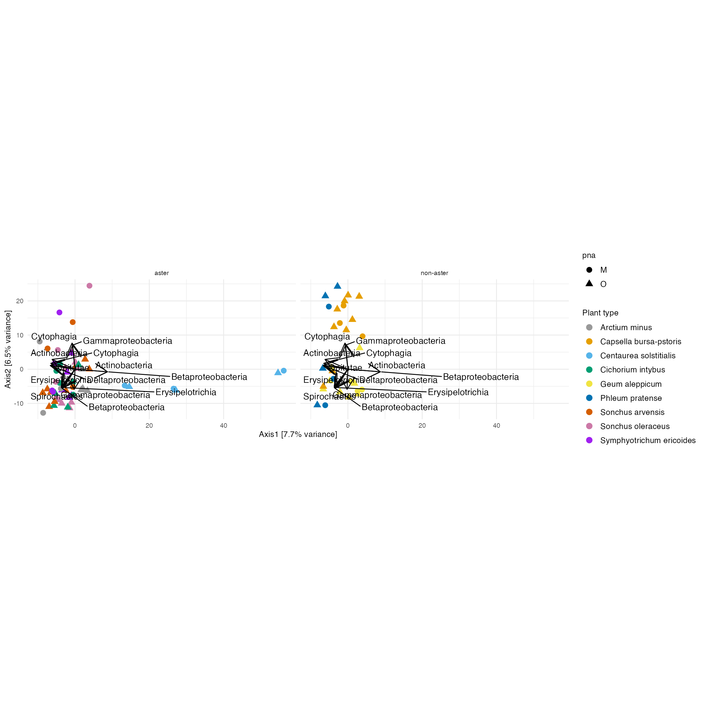
Figure 2: The biplot from the PCA after the truncated-rank transformation. The shape denotes universal (O) and Asteraceae-modified (M) pPNA types, respectively. Facet denotes Asteraceae or non-Asteraceae plants. Actinobac- teria and Betaproteobacteria dominate in outliers Centaurea solstitialis in the positive direction of the first axis. The second axis explains the plant microbiome variability in non-Asteraceae specimens.

Pratheepa Jeganathan

04 August, 2021