Section 6: VISUALIZATIONS FOR HETEROGENEOUS DATA
Pratheepa Jeganathan
04 August, 2021
06_visualization.Rmd
library(phyloseq)
library(tidyverse)
library(genefilter) #KOverA
library(pheatmap)
devtools::load_all()
theme_set(theme_minimal())
theme_update(
  text = element_text(size = 10),
  legend.text = element_text(size = 10)
)
Data
data("psE_BARBI")
threshold <- kOverA(2, A = 25)
psE_BARBI <- phyloseq::filter_taxa(
  psE_BARBI,
  threshold, TRUE)

psE_BARBI
## phyloseq-class experiment-level object
## otu_table() OTU Table: [ 1418 taxa and 86 samples ]
## sample_data() Sample Data: [ 86 samples by 16 sample variables ]
## tax_table() Taxonomy Table: [ 1418 taxa by 6 taxonomic ranks ]
## phy_tree() Phylogenetic Tree: [ 1418 tips and 1417 internal nodes ]
ps <- psE_BARBI
rm(psE_BARBI)
ps <- prune_taxa(taxa_sums(ps) > 0, ps)
ps
## phyloseq-class experiment-level object
## otu_table() OTU Table: [ 1418 taxa and 86 samples ]
## sample_data() Sample Data: [ 86 samples by 16 sample variables ]
## tax_table() Taxonomy Table: [ 1418 taxa by 6 taxonomic ranks ]
## phy_tree() Phylogenetic Tree: [ 1418 tips and 1417 internal nodes ]Edit specimen names
We edit specimen names and identify Asteraceae and non-Asteraceae plants.
sam_names <- str_replace(sample_names(ps), "E106", "E-106")
sam_names <- str_replace(sam_names, "_F_filt.fastq.gz", "")
sam_names <- str_replace(sam_names, "Connor-", "E")
sample_names(ps) <- sam_names
sample_data(ps)$X <- sam_names
sample_data(ps)$unique_names <- sam_names
aster <- c("142","143","15","ST","22","40")
non_aster <- c("33", "71", "106")

paired_aster <- c("E-142-1", "E142-1", "E-142-5", "E142-5", "E-142-10", "E142-10", "E-143-2", "E143-2", "E-143-7", "E143-7", "E-15-1", "E15-1", "ST-CAZ-4-R-O", "ST-CAZ-4-R-M", "ST-SAL-22-R-O", "ST-SAL-22-R-M", "ST-TRI-10-R-O", "ST-TRI-10-R-M")
paired_non_aster <- c("E33-7", "E-33-7", "E33-8", "E-33-8", "E33-9", "E-33-9", "E71-10", "E-71-10","E71-2","E-71-2" ,"E71-3", "E-71-3", "E106-1", "E-106-1", "E106-3", "E-106-3", "E106-4", "E-106-4")
paired_specimens <- c(paired_aster, paired_non_aster)
# We will use 9 colors for 9 different plants
plant_colors <- c("#999999", "#E69F00", "#56B4E9", "#009E73", "#F0E442", "#0072B2", "#D55E00", "#CC79A7", "purple")
Barplots for estimates of \(p_{j}=(p_{i,j}, i=1\ldots m)\)
For this section, we consider the example data set after the contamination removal. There are 1418 taxa in 86 samples. We compute the relative abundance of ASVs in each specimen. Then, we remove ASVs corresponding to the Class with less than five ASVs.
ps_ra <- transform_sample_counts(
  ps,
  function(x){x / sum(x)}
  )
remov_asvs <- names(table(tax_table(ps)[, "Class"]))[which(table(tax_table(ps)[, "Class"]) <= 5)]

ps_ra <- subset_taxa(ps_ra,
                     !(Class %in% remov_asvs) & !is.na(Class)
                     )
ps_temp <- subset_taxa(ps,
                       !(Class %in% remov_asvs) & !is.na(Class)
                       )
ps_temp
## phyloseq-class experiment-level object
## otu_table() OTU Table: [ 1342 taxa and 86 samples ]
## sample_data() Sample Data: [ 86 samples by 16 sample variables ]
## tax_table() Taxonomy Table: [ 1342 taxa by 6 taxonomic ranks ]
## phy_tree() Phylogenetic Tree: [ 1342 tips and 1341 internal nodes ]We plot the distribution of relative abundance of each Phylum in specimens faceted by Class. We can use the barplots to compare difference in scale and distribution of Phylum in universal and Aster-modified pPNA types.
phylum_order_by_num_asv <- sort(
  table(tax_table(ps_temp)[, "Phylum"]),
  decreasing = TRUE
  )

# most number of ASVs are from Proteobacteria
ps_proteobacteria <- subset_taxa(
  ps_temp,
  Phylum %in% c("Proteobacteria")
  )

ps_ra_proteobacteria <- subset_taxa(
  ps_ra,
  Phylum %in% c("Proteobacteria")
  )

plot_abundance <- function(
  physeq,
  title = "",
  Facet = "Class",
  Color = "Phylum"){
    mphyseq <- psmelt(physeq)
    mphyseq <- subset(
      mphyseq,
      Abundance > 0
      )
    ggplot(
      data = mphyseq,
      mapping = aes_string(
        x = "pna",
        y = "Abundance",
        color = Color,
        fill = Color)
      ) +
      geom_violin(fill = NA) +
      geom_point(
        size = 1,
        alpha = 0.3,
        position = position_jitter(width = 0.3)
        ) +
      facet_wrap(facets = Facet) +
      scale_y_log10() +
      ggtitle(title)+
      xlab("pPNA type")+
      theme(legend.position="none",
            plot.title = element_text(hjust = 0.5))
}
plot_abundance(
  subset_samples(
    ps_proteobacteria,
    Type == "aster"),
  title = "Asteraceae") +
  ylab("Abundance")
plot_abundance(
  subset_samples(
    ps_ra_proteobacteria,
    Type == "aster"),
  title = "Asteraceae") +
  ylab("Relative abundance")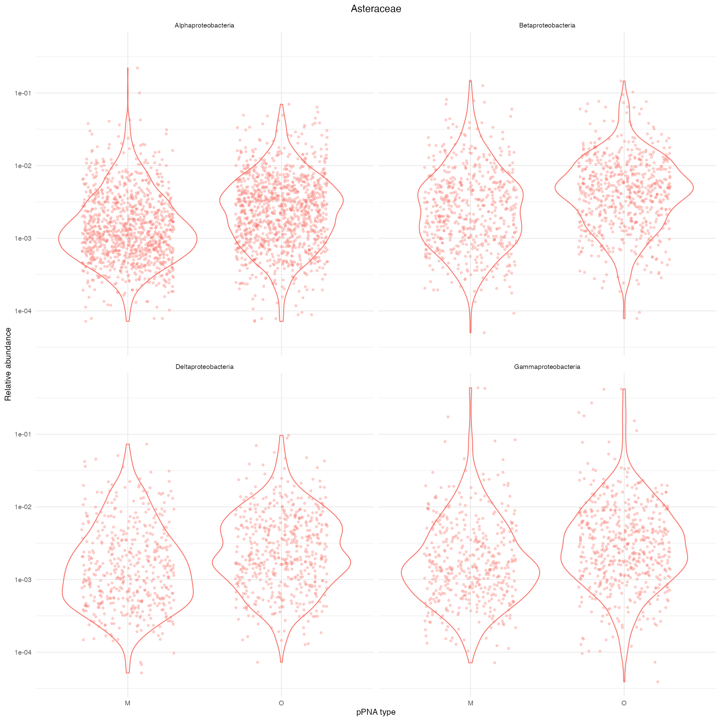
Supplementary Figure 6: Distribution of relative abundance of four different Classes of Proteobacteria in Asteraceae plants. O and M denote universal and Asteraceae-modified pPNA types, respectively.
plot_abundance(
  subset_samples(
    ps_proteobacteria,
    Type == "non-aster"),
  title = "non-Asteraceae"
  )
plot_abundance(
  subset_samples(
    ps_ra_proteobacteria,
    Type == "non-aster"),
  title = "non-Asteraceae") +
  ylab("Relative abundance")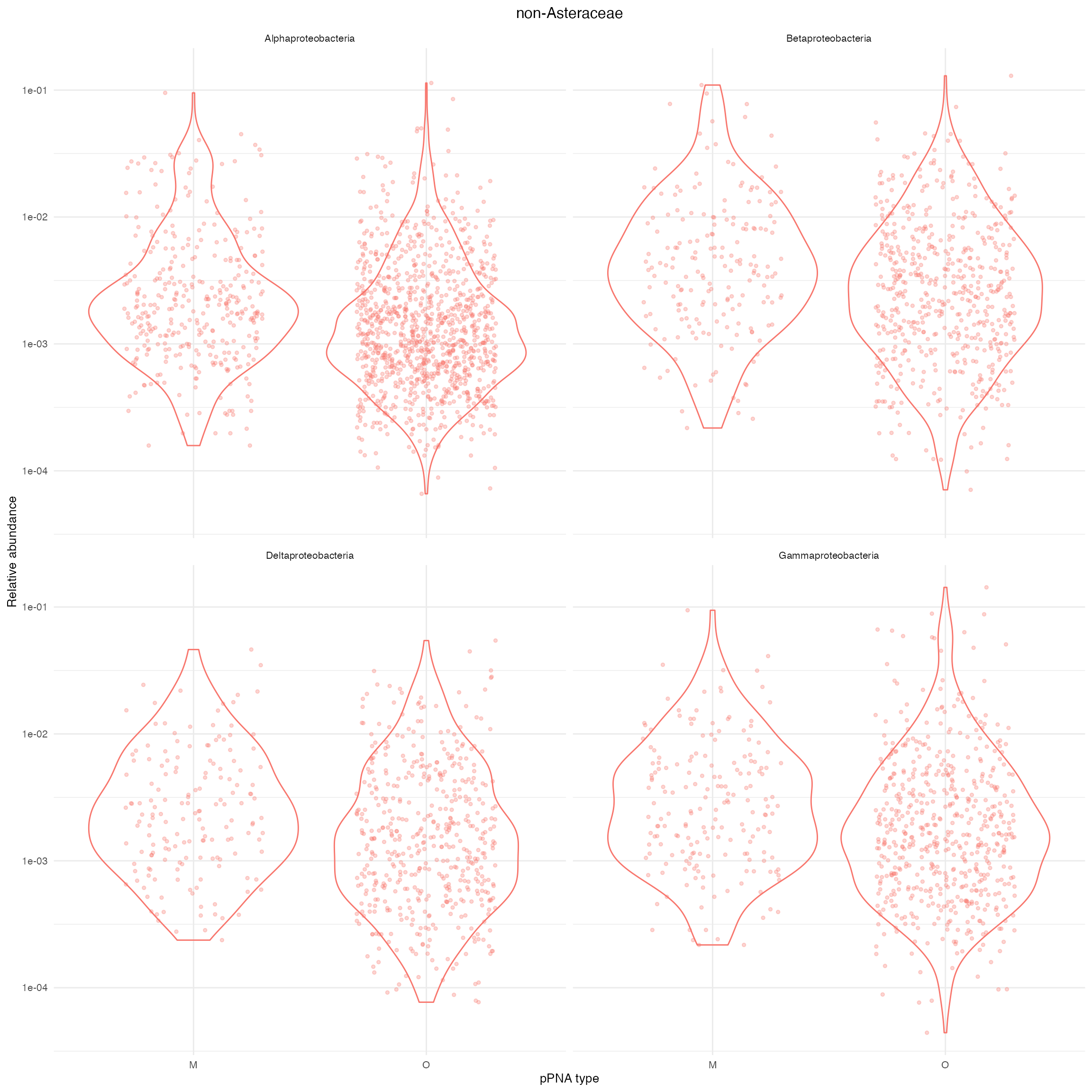
Supplementary Figure 7: Distribution of relative abundance of four different Classes of Proteobacteria in non- Asteraceae plants. O and M denote universal and Asteraceae-modified pPNA types, respectively.
Heatmaps
We plot the heatmap of Anscombe’s transformed values.
data("ps_ans")
# do use asinh transformation
ps_top <- ps_ans

# choose top 30 ASVs in endo specimens for heatmap
top <- names(
  sort(
    taxa_sums(
      ps_top
      ),
    decreasing=TRUE
    )
  )[1:30]

ps_top <- prune_taxa(
  top,
  ps_top
  )

or <- order(
  taxa_sums(ps_top),
  decreasing=TRUE
  )[1:30]

ass <- otu_table(ps_top) %>%
  data.frame()

colnames(ass) <- sample_names(ps_top)

tx <- tax_table(ps_top) %>%
  data.frame()

tx <- dplyr::mutate(tx,
                    usename = paste0(
                      "ASV_",
                      seq(1, ntaxa(ps_top)),
                      "_",
                      tax_table(ps_top)[, "Class"]
                      ),
                    rnames = taxa_names(ps_top)
                    )

ass <- ass[or, ]
rownames(ass) <- tx$usename[or]

df <- sample_data(ps_top) %>%
  data.frame()

df <- df[ , c(
  "Type",
  "species_names",
  "pna",
  "unique_names"
  )]

colnames(df)[which(colnames(df) == "species_names")] <- "plant_type"

df <- with(
  df,
  df[order(Type, plant_type, pna, unique_names),]
  )

ass <- ass[, df$unique_names]

df <- dplyr::select(
  df,
  -unique_names
  )

Type <- c("royalblue3", "seagreen1")
names(Type) <- levels(df$Type)
plant_type <- plant_colors
names(plant_type) <- levels(df$plant_type)
pna <- c("orange3", "palegreen4")
names(pna) <- levels(df$pna)

ann_colors <-  list(
  Type = Type,
  plant_type = plant_type,
  pna = pna
  )

pheatmap(
  ass,
  annotation_col = df,
  cluster_rows = FALSE,
  cluster_cols = FALSE,
  fontsize_row = 14,
  fontsize_col = 10,
  annotation_colors = ann_colors
  )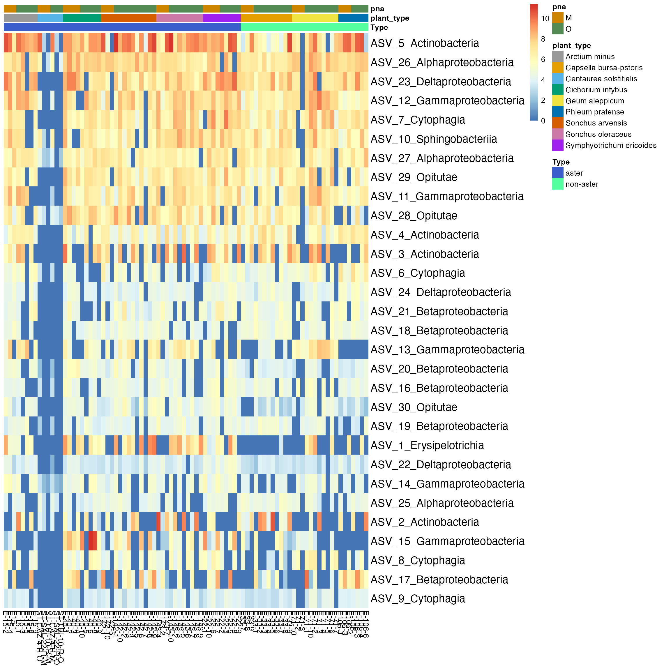
Figure 3: Thirty most abundant ASVs were selected in all specimens. Taxa are labeled by Class on rows, and specimens are on the columns of the heatmap. Some specimens from Centaurea solstitialis plant have the most abundant ASVs of the Class Actinobacteria, Alphaproteobacteria, Sphingobacteria, and Gammaproteobacteria.