Section 7: MULTIVARIATE AND NETWORK ANALYSES
Pratheepa Jeganathan
04 August, 2021
07_multivariate_and_network_analysis.Rmd
library(phyloseq)
library(tidyverse)
library(genefilter) #KOverA
library(ggrepel) # geom_text_repel
library(randomcoloR)# distinctColorPalette(n)
library(adaptiveGPCA)
library(igraph)
library(phyloseqGraphTest)
devtools::load_all()
theme_set(theme_minimal())
theme_update(
  text = element_text(size = 10),
  legend.text = element_text(size = 10)
)
Data
data("psE_BARBI")
threshold <- kOverA(2, A = 25)
psE_BARBI <- phyloseq::filter_taxa(
  psE_BARBI,
  threshold, TRUE)

psE_BARBI
## phyloseq-class experiment-level object
## otu_table() OTU Table: [ 1418 taxa and 86 samples ]
## sample_data() Sample Data: [ 86 samples by 16 sample variables ]
## tax_table() Taxonomy Table: [ 1418 taxa by 6 taxonomic ranks ]
## phy_tree() Phylogenetic Tree: [ 1418 tips and 1417 internal nodes ]
ps <- psE_BARBI
rm(psE_BARBI)
ps <- prune_taxa(taxa_sums(ps) > 0, ps)
ps
## phyloseq-class experiment-level object
## otu_table() OTU Table: [ 1418 taxa and 86 samples ]
## sample_data() Sample Data: [ 86 samples by 16 sample variables ]
## tax_table() Taxonomy Table: [ 1418 taxa by 6 taxonomic ranks ]
## phy_tree() Phylogenetic Tree: [ 1418 tips and 1417 internal nodes ]Edit specimen names
We edit specimen names and identify Asteraceae and non-Asteraceae plants.
sam_names <- str_replace(sample_names(ps), "E106", "E-106")
sam_names <- str_replace(sam_names, "_F_filt.fastq.gz", "")
sam_names <- str_replace(sam_names, "Connor-", "E")
sample_names(ps) <- sam_names
sample_data(ps)$X <- sam_names
sample_data(ps)$unique_names <- sam_names
aster <- c("142","143","15","ST","22","40")
non_aster <- c("33", "71", "106")

paired_aster <- c("E-142-1", "E142-1", "E-142-5", "E142-5", "E-142-10", "E142-10", "E-143-2", "E143-2", "E-143-7", "E143-7", "E-15-1", "E15-1", "ST-CAZ-4-R-O", "ST-CAZ-4-R-M", "ST-SAL-22-R-O", "ST-SAL-22-R-M", "ST-TRI-10-R-O", "ST-TRI-10-R-M")
paired_non_aster <- c("E33-7", "E-33-7", "E33-8", "E-33-8", "E33-9", "E-33-9", "E71-10", "E-71-10","E71-2","E-71-2" ,"E71-3", "E-71-3", "E106-1", "E-106-1", "E106-3", "E-106-3", "E106-4", "E-106-4")
paired_specimens <- c(paired_aster, paired_non_aster)
# We will use 9 colors for 9 different plants
plant_colors <- c("#999999", "#E69F00", "#56B4E9", "#009E73", "#F0E442", "#0072B2", "#D55E00", "#CC79A7", "purple")
7.1 Ordination
Multidimensional scaling (MDS) with weighted unifrac
ps_log <- transform_sample_counts(
  ps,
  function(x) log(1 + x)
  )

out.wuf.log <- ordinate(
  ps_log,
  method = "MDS",
  distance = "wunifrac"
  )

evals <- out.wuf.log$values$Eigenvalues

mds_wuni <- plot_ordination(
  ps_log,
  out.wuf.log,
  color = "species_names",
  shape = "pna"
  ) +
  labs(
    col = "Plant type"
    ) +
  coord_fixed(
    sqrt(evals[2] / evals[1])
    ) +
  scale_colour_manual(
    values = plant_colors
    ) +
  facet_grid(~Type) +
  geom_point(size = 3)

# adding only paired-specimen names
df_paired <- mds_wuni$data %>%
  dplyr::filter(
    unique_names %in% paired_specimens
    )

mds_wuni +
  geom_text_repel(
    data = df_paired,
    aes(
      x = Axis.1,
      y = Axis.2,
      label = unique_names
      ),
    color = "black"
    )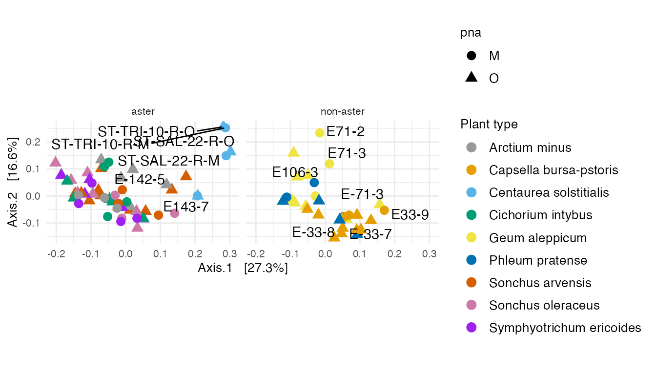
Supplementary Figure 8: Multidimensional scaling (MDS) with weighted unifrac distance on all specimens.
We see that Centaurea solstitialis specimens are outlier that were sampled in a field across three countries, while other plants are grown from seeds. We label the paired specimens in all plants. The paired specimens are relatively close to each other, except (E-143-7, E143-7), (E-142-5, E142-5), (E-71-2, E71-2), and (E-71-3, E71-3) that are in positive and negative axes of the first two principal axes.
Fitzpatrick et al. (2018) concluded that there is no effect in within and between specimen bacterial diversity when they used universal or Aster-modified pPNA types.
The above Figure shows that specimens from the aster plants that are paired with universal or Aster-modified pPNA types make clusters.
MDS with BC
An MDS plot using Bray-Curtis distance between specimens.
out.bc.log <- ordinate(
  ps_log,
  method = "MDS",
  distance = "bray"
  )

evals <- out.bc.log$values$Eigenvalues

mds_bc <- plot_ordination(
  ps_log,
  out.bc.log,
  color = "species_names",
  shape = "pna"
  ) +
  coord_fixed(
    sqrt(evals[2] / evals[1])
    ) +
  labs(
    col = "Plant type",
    shape = "pna"
    ) +
  scale_colour_manual(
    values = plant_colors
    ) +
  facet_grid(~Type) +
  geom_point(size=3)

df_paired <- mds_bc$data %>%
  dplyr::filter(
    unique_names %in% paired_specimens
    )

mds_bc +
  geom_text_repel(
    data = df_paired,
    aes(x = Axis.1,
        y = Axis.2,
        label = unique_names
        ),
    color = "black"
    )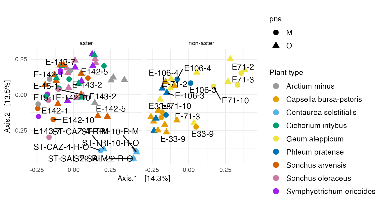
The ordination of specimens in MDS with BC is similar to MDS with weighted unifrac.
DPCoA
A DPCoA plot incorporates phylogenetic information.
The DPCoA specimens positions can be interpreted with respect to the ASVs coordinates in this display.
data("ps_ans")
out.dpcoa.log <- ordinate(
  ps_ans,
  method = "DPCoA"
  )

evals <- out.dpcoa.log$eig

dpcoa_sam <- plot_ordination(
  ps_ans,
  out.dpcoa.log,
  color = "species_names",
  shape = "pna"
  ) +
  coord_fixed(
    sqrt(evals[2] / evals[1])
    ) +
  labs(
    col = "Plant type",
    shape = "pna"
    ) +
  scale_colour_manual(
    values = plant_colors
    ) +
  facet_grid(~Type) +
  geom_point(size = 3)

df_paired <- dpcoa_sam$data %>%
  dplyr::filter(
    unique_names %in% paired_specimens
    )

dpcoa_sam +
  geom_text_repel(
    data = df_paired,
    aes(
      x = CS1,
      y = CS2,
      label = unique_names
      ),
    color = "black"
    )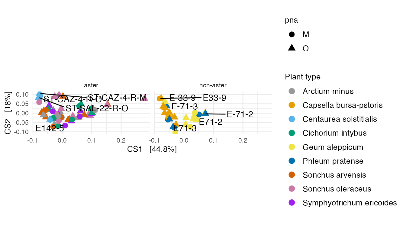
Supplementary Figure 9: (A) A DPCoA plot that incorporates phylogenetic information.
dpcoa_taxa <- plot_ordination(
  ps_ans,
  out.dpcoa.log,
  type = "species",
  color = "Class"
  )


df_taxa <- dplyr::filter(
  dpcoa_taxa$data,
  (CS1 > 0.63 | CS1 < -0.14 | CS2 > 0.29 | CS2 < -0.13) & (
    !is.na(Class)
    )
  )

dpcoa_taxa$data <- df_taxa

dpcoa_taxa +
  coord_fixed(
    sqrt(evals[2] / evals[1])
    ) +
  geom_point(size = 2) +
  scale_color_manual(
    values = distinctColorPalette(
      length(
        unique(
          tax_table(ps_ans)[, "Class"]
          )
        )
      )
    )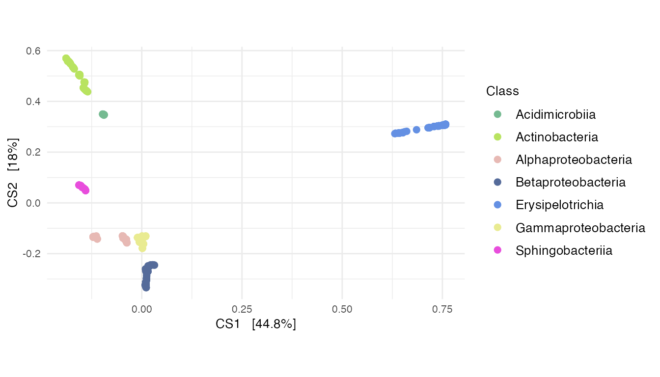
Supplementary Figure 9: (A) A DPCoA plot that incorporates phylogenetic information.
7.2 Integrating the phylogenetic tree into the analyses
Adaptive gPCA
pp <- processPhyloseq(
  ps
  )
out.agpca <- adaptivegpca(
  pp$X,
  pp$Q,
  k = 2
  )

agPCA_samples <- ggplot(
  data.frame(
    out.agpca$U,
    sample_data(ps)
    )
  ) +
    geom_point(
      aes(x = Axis1,
          y = Axis2,
          color = species_names,
          shape = pna),
      size = 3
      ) +
  labs(
    x = "Axis 1",
    y = "Axis 2",
    col = "Plant type"
    ) +
  scale_colour_manual(
    values = plant_colors
    ) +
  facet_grid(~ Type)

agPCA_samples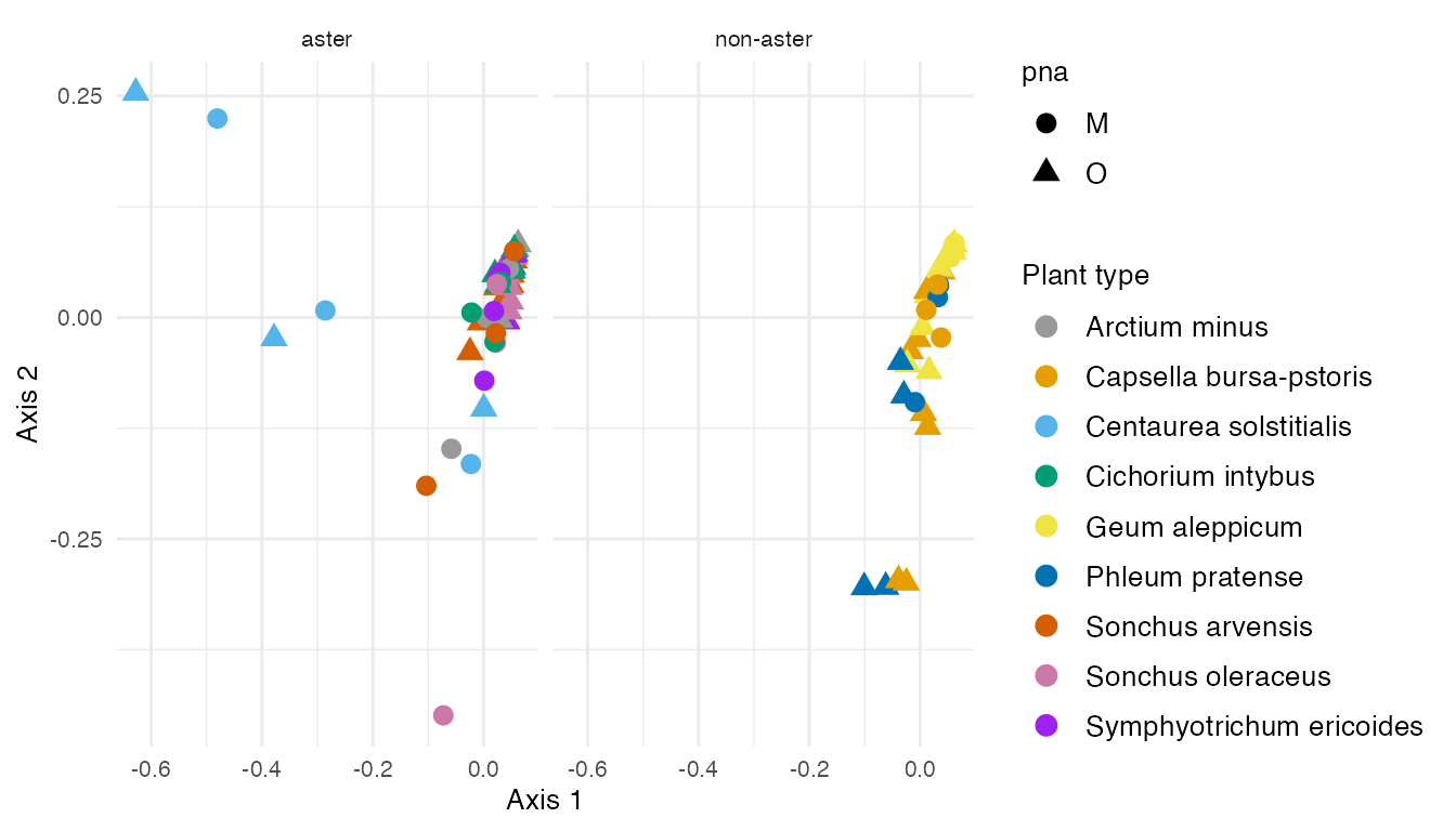
Figure 4: The results from adaptive gPCA reveal Centaurea solstitialis specimens are outliers among Asteraceae plants in the left of Axis 1. Axis 2 explains the microbial variability in plant types.
agPCA_asv <- ggplot(
  data.frame(
    out.agpca$QV,
    tax_table(ps)
    )
  ) +
    geom_point(
      aes(
        x = Axis1,
        y = Axis2,
        color = Class
        ),
      size = 3
      ) +
    xlab(
      "Axis 1"
      ) +
  ylab(
    "Axis 2"
    )

main_class <- c("Bacilli",
                "Actinobacteria",
                "Cytophagia",
                "Gammaproteobacteria",
                "Betaproteobacteria",
                "Deltaproteobacteria",
                "Alphaproteobacteria",
                "Opitutae")

df_taxa <- dplyr::filter(
  agPCA_asv$data,
  Class %in% main_class
  )

agPCA_asv$data <- df_taxa

agPCA_asv <- agPCA_asv +
  scale_color_manual(
    values = distinctColorPalette(
      length(
        unique(
          tax_table(ps_ans)[, "Class"])
        )
      )
    )
agPCA_asv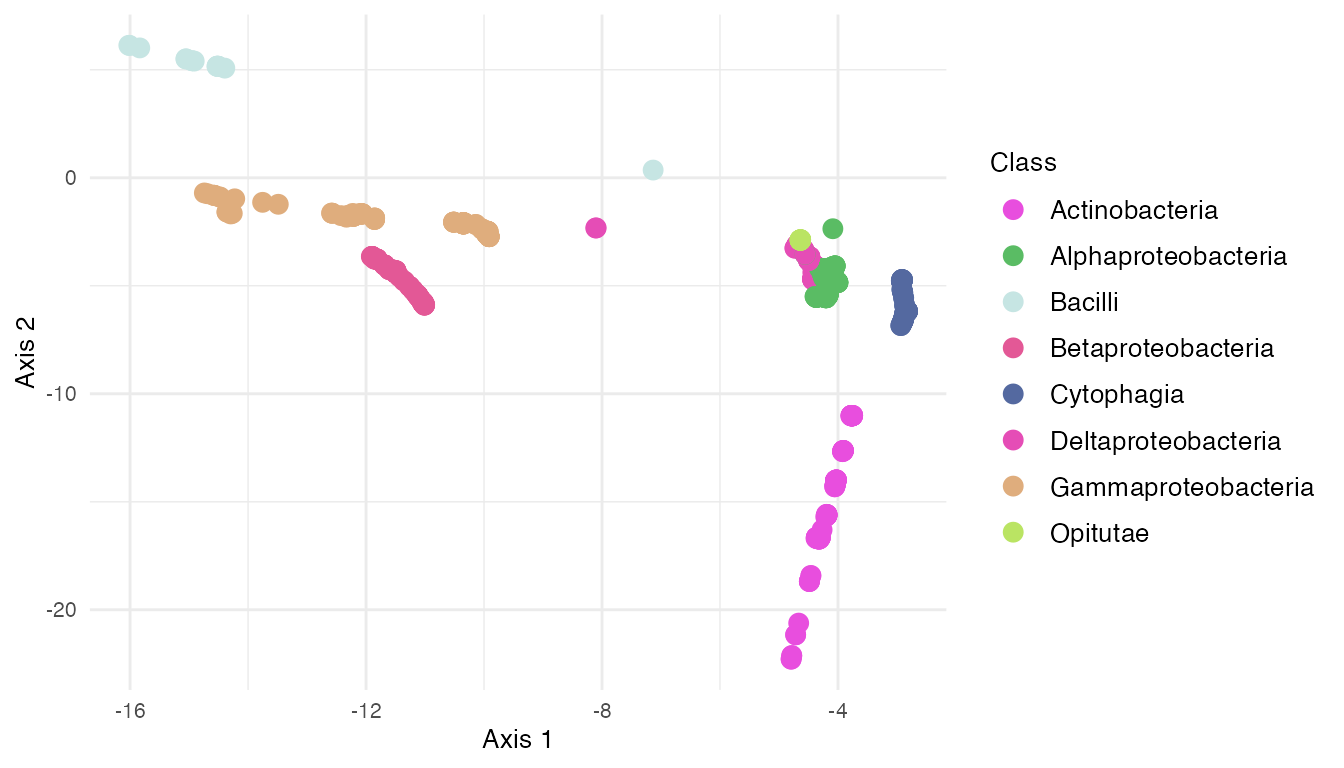
Centaurea solstitialis specimens are outliers among Asteraceae plants on the left of Axis 1. Axis 2 explains the microbial variability in plant types.
7.3 Correspondence analysis
ps_ca <- ps
out.ca <- ordinate(
  ps_ca,
  method = "CCA"
  )

evals <- out.ca$CA$eig
evals_prop <- evals/sum(evals)

ca_plot <- plot_ordination(
  ps_ca,
  out.ca,
  type = "sample",
  color = "species_names",
  shape = "pna") +
  labs(
    col = "Plant type",
    shape = "pna"
    ) +
  scale_color_manual(
    values = plant_colors
    ) +
  facet_grid(~Type) +
  geom_point(size=2) +
  geom_jitter()+
  coord_fixed(0.4) +
  theme_update(
    text = element_text(size = 10),
    legend.text = element_text(size = 10),
    panel.spacing = unit(2, "lines")
)


ca_plot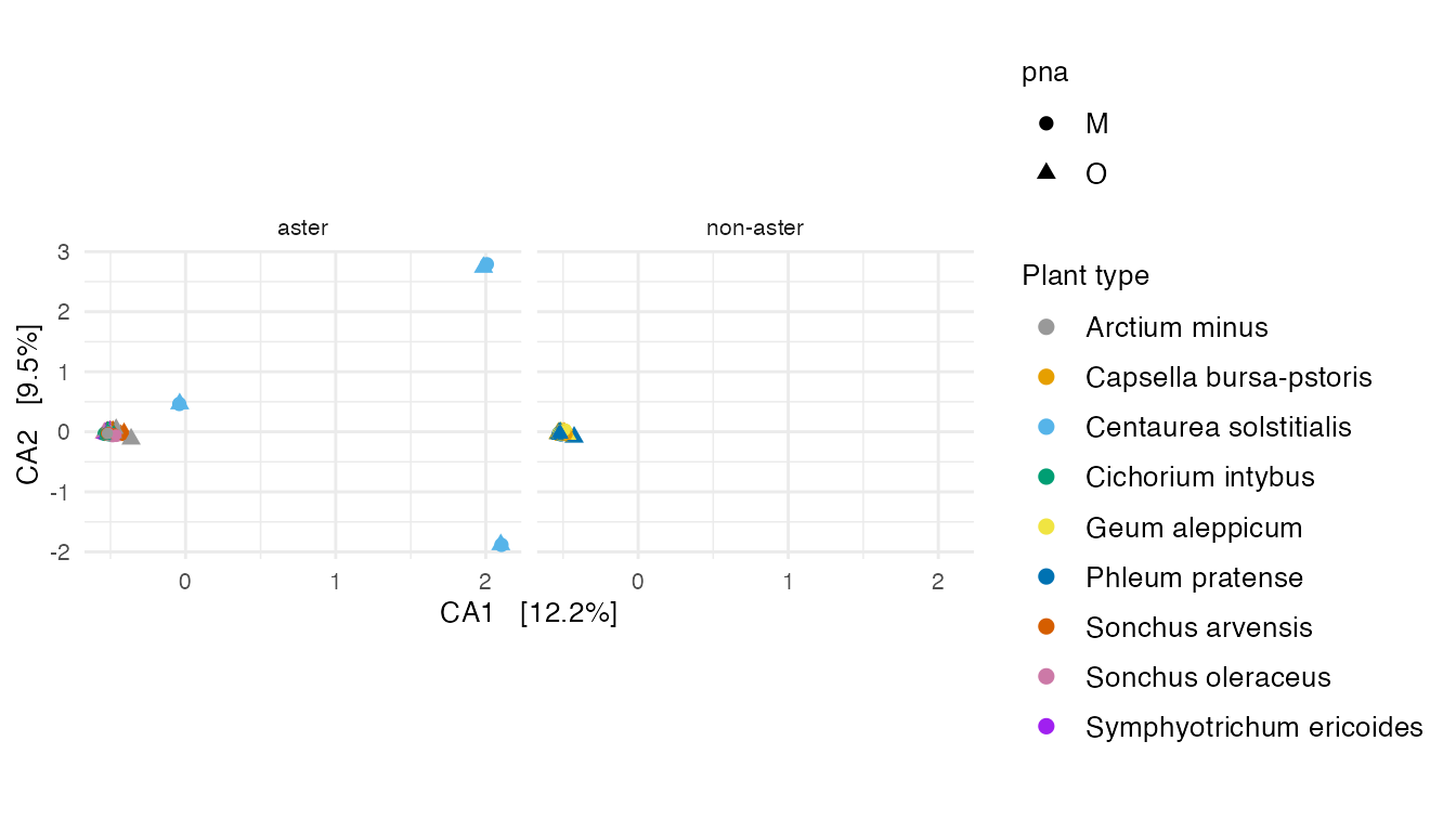
Figure 5: Correspondence analysis of all plant specimens. (A)
ca_plot_taxa <- plot_ordination(
  ps_ca,
  out.ca,
  type = "species",
  color = "Class"
  )

main_class <- c("Bacilli",
                "Actinobacteria",
                "Cytophagia",
                "Gammaproteobacteria",
                "Betaproteobacteria",
                "Deltaproteobacteria",
                "Alphaproteobacteria",
                "Opitutae",
                "Sphingobacteriia")

df_taxa <- dplyr::filter(
  ca_plot_taxa$data,
  Class %in% main_class
  )

df_taxa$Class <- factor(df_taxa$Class)

ca_plot_taxa$data <- df_taxa

ca_plot_taxa <- ca_plot_taxa +
  coord_fixed(0.4) +
  labs(col = "Class") +
  geom_point(size=3) +
  geom_jitter() +
  scale_color_manual(
    values = distinctColorPalette(
      length(
        unique(
          main_class
          )
        )
      )
    )

ca_plot_taxa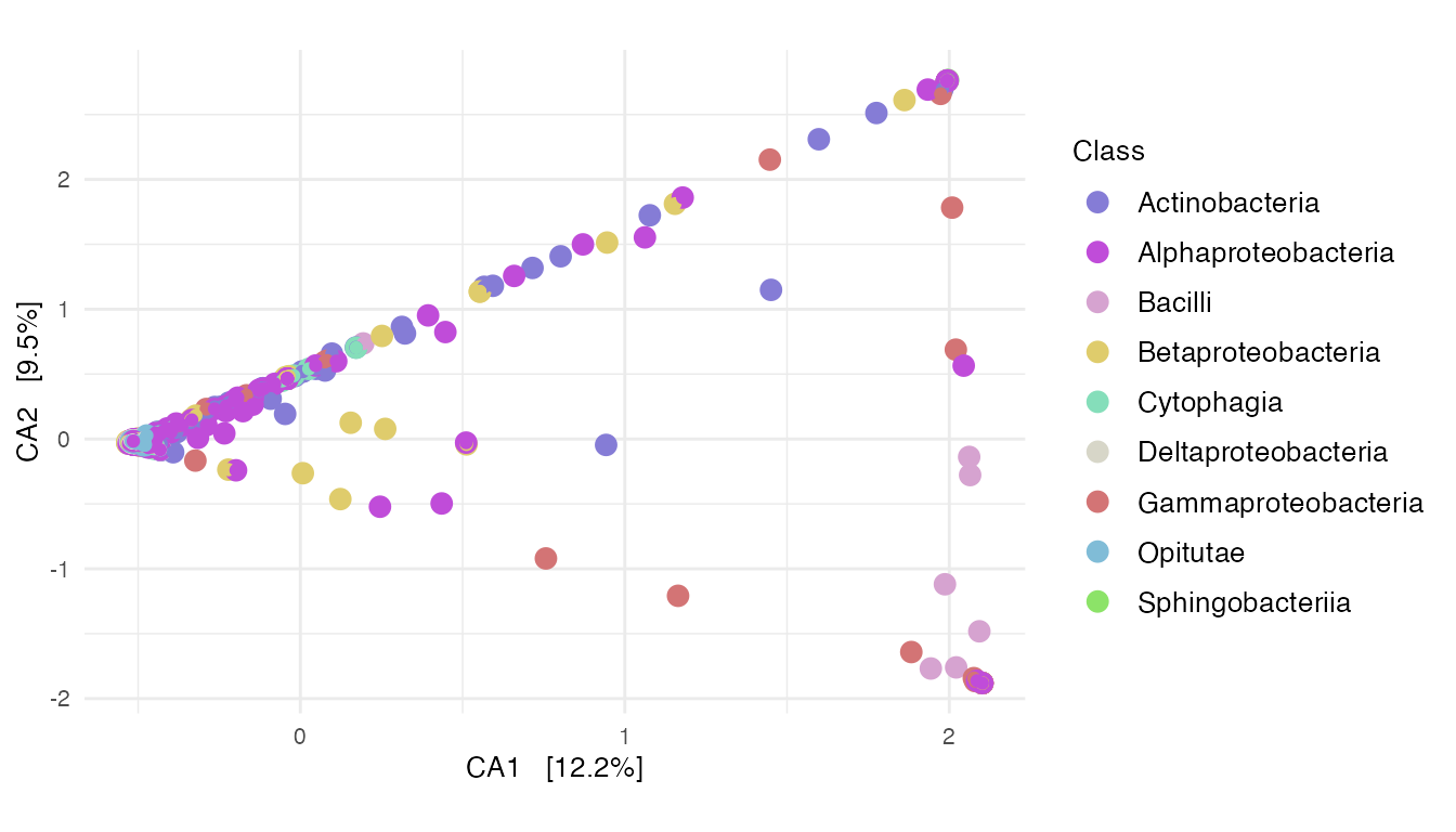
Figure 5: Correspondence analysis of all plant specimens. (B)
7.4 Network analysis
Network analysis on paired specimens
ps <- subset_samples(
  ps,
  unique_names %in% paired_specimens
  )
ps <- prune_taxa(
  taxa_sums(ps) > 0,
  ps
  )
ps
## phyloseq-class experiment-level object
## otu_table() OTU Table: [ 1348 taxa and 36 samples ]
## sample_data() Sample Data: [ 36 samples by 16 sample variables ]
## tax_table() Taxonomy Table: [ 1348 taxa by 6 taxonomic ranks ]
## phy_tree() Phylogenetic Tree: [ 1348 tips and 1347 internal nodes ]
net <- make_network(
  ps,
  max.dist = 0.8
  )

sampledata <- sample_data(ps) %>%
  data.frame()

V(net)$unique_names <- sampledata[names(V(net)), "unique_names"]
V(net)$pna <- sampledata[names(V(net)), "pna"]
V(net)$species_names <- sampledata[names(V(net)), "species_names"]

p_net <- plot_network(
  net,
  ps,
  color = "species_names",
  shape = "pna"
  ) +
  labs(
    col = "Species names"
    ) +
  scale_colour_manual(
    values = plant_colors
    )
p_net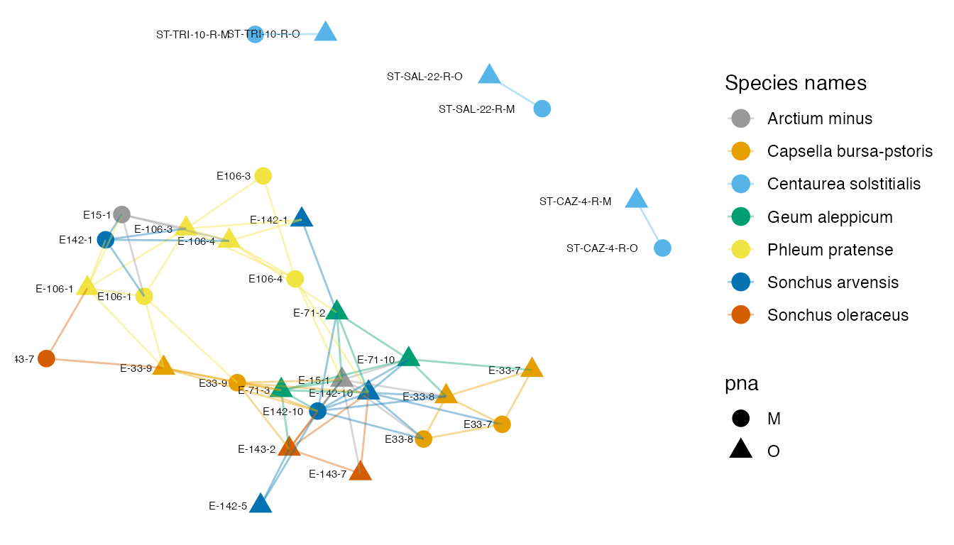
Supplementary Figure 10: A network created by thresholding the Jaccard dissimilarity matrix at 0.8.
Graph-based two-sample tests
We first perform a test using an Minimum spanning tree (MST) with Jaccard dissimilarity. We want to know whether the universal or Asteraceae-modified pPNAs come from the same distribution in paired-specimens.
Since there is a grouping in the data by specimen, we can’t simply permute all the labels, we need to maintain this nested structure – this is what the grouping argument does. Here we permute the pna labels but keep the plant type structure intact.
set.seed(15)
gt <- graph_perm_test(
  ps,
  sampletype = "pna",
  grouping = "unique_names",
  distance = "jaccard",
  type = "mst")
gt$pval
## [1] 0.882This test has a larger p-value, and we do not reject the null hypothesis that the paired-specimens come from the same distribution.
This result mirrors the observations from the PCA after the truncated-rank transformation, adaptive gPCA, MDS, and DPCoA that paired-specimens have similar microbial variability.