Vignette for bootLong: The Block Bootstrap Method for Longitudinal Microbiome Data
Pratheepa Jeganathan and Susan Holmes
jpratheepa31@gmail.combootLong.RmdMicrobiome data consist of the frequency of higher resolution amplicon sequence variants (ASVs) in each biological sample, clinical and demographic information about biological samples, phylogenetic tree, taxonomy table. Our bootLong package requires phyloseq for the entire workflow.
In this workflow, we provide differential abundance analysis for longitudinal microbiome data. In addition, we provide statistical tools to explore the sampling schedule and within-subject dependency for each ASV.
A preprint describing the method is available in stat arXiv.
Install R and RStudio. Open this Rmd file in RStudio. Then run the following code to install all required packages.
Install and load required packages
Install
pkgs <- c("ggplot2", "dplyr", "tidyr",
          "phyloseq", "limma", "ashr",
          "gridExtra", "MASS",
          "geeM", "BiocParallel",
          "doParallel", "parallel","magrittr",
          "joineR", "DESeq2", "grid", "devtools")


BiocManager::install(setdiff(pkgs, installed.packages()), update = TRUE)

#devtools::install_github("PratheepaJ/bootLong")
load
library(ggplot2)
library(dplyr)
library(tidyr)
library(phyloseq)
library(limma)
library(ashr)
library(gridExtra)
library(MASS)
library(geeM)
library(BiocParallel)
library(doParallel)
library(parallel)
library(magrittr)
library(joineR)
library(DESeq2)
library(grid)
#library(bootLong)
# library(R.utils)
devtools::load_all(".")
Set the computational resources
We need to specify the number of cores for subsampling method and block bootstrap method.
ncores <- as.integer(Sys.getenv("SLURM_NTASKS"))
if(is.na(ncores)) ncores <- parallel::detectCores()
ncores
## [1] 4Specify setting_name to save the results.
lC1 and lC2 are the minumum and the maximum block length for subsampling method.
## [1] 2## [1] 2The plots can be modified using your preferred theme, legends, etc. For example, set.theme can be changed to have point size 10.
theme_set(theme_bw())
set.theme <- theme_update(panel.border = element_blank(),
                    panel.grid = element_line(size = .8),
                    axis.ticks = element_blank(),
                    legend.title = element_text(size = 8),
                    legend.text = element_text(size = 8),
                    axis.text = element_text(size = 8),
                    axis.title = element_text(size = 8),
                    strip.background = element_blank(),
                    strip.text = element_text(size = 8),
                    legend.key = element_blank(),
    plot.title = element_text(hjust = 0.5))
Load the phyloseq or create a phyloseq
Follow the tutorials to creating phyloseq.
Load the example dataset stored as a phyloseq in this package (or use your own phyloseq or created as a phyloseq)
Exploratory analysis
Summary
After loading the phyloseq, we recommend to check the variable names and some summary for each variable in the sample table: sample_data(ps).
In the example data psSim, we have SubjectID, SampleID, Time, Preterm variables. Preterm is the covariate.
## [1] "SubjectID" "Group" "SampleID" "Time"##
## 1 2 3 4 5 6 7 8 9 10
## Cas1 1 1 1 1 1 1 1 1 1 1
## Cas10 1 1 1 1 1 1 1 1 1 1
## Cas2 1 1 1 1 1 1 1 1 1 1
## Cas3 1 1 1 1 1 1 1 1 1 1
## Cas4 1 1 1 1 1 1 1 1 1 1
## Cas5 1 1 1 1 1 1 1 1 1 1
## Cas6 1 1 1 1 1 1 1 1 1 1
## Cas7 1 1 1 1 1 1 1 1 1 1
## Cas8 1 1 1 1 1 1 1 1 1 1
## Cas9 1 1 1 1 1 1 1 1 1 1
## Con1 1 1 1 1 1 1 1 1 1 1
## Con10 1 1 1 1 1 1 1 1 1 1
## Con2 1 1 1 1 1 1 1 1 1 1
## Con3 1 1 1 1 1 1 1 1 1 1
## Con4 1 1 1 1 1 1 1 1 1 1
## Con5 1 1 1 1 1 1 1 1 1 1
## Con6 1 1 1 1 1 1 1 1 1 1
## Con7 1 1 1 1 1 1 1 1 1 1
## Con8 1 1 1 1 1 1 1 1 1 1
## Con9 1 1 1 1 1 1 1 1 1 1## Case Control
## 100 100Sampling schedule
We can visualize the sampling schedule for each subject and facet by different conditions. The plot can be modified using your preferred theme. For example, the legend title can be changed from Preterm to Group, levels of Preterm can be changed to Term and Preterm, etc.
The sampling schedule will be used to choose the \(\omega\) repeated observations from each subject for the subsampling procedure. So that we can use \(W = q - \omega +1\) overlapping subsamples to find the optimal block length for the full data with all repeated observations \(q\).
sample_data(ps)$Group <- as.factor(sample_data(ps)$Group)

p <- plotSamplingSchedule(ps,
  time_var = "Time",
  subjectID_var = "SubjectID",
  main_factor = "Group",
  theme_manual = set.theme)

p <- p +
  scale_color_discrete(name  ="Group",
    breaks=c("Case", "Control"),
    labels=c("Case", "Control"))
p + ylab("Subject ID")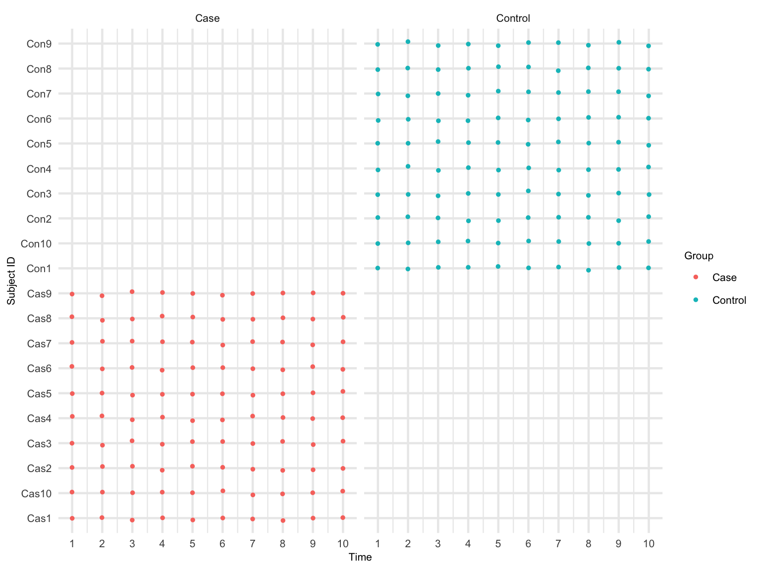
Sampling schedule
# fileN <- paste0("sampling_schedule_", setting_name, ".eps")
#ggsave(fileN, plot = p, width = 8, height = 5.5)
Based on Figure @ref(fig:plot-sam-sch), in order to make at least five (\(W = 5\)) overlapping subsamples, we should choose \(\omega = .6\) (\(\omega\) cannot be more than .6). The maximum repeated observations from each subject for the subsample is \(10 \times .6 = 6\). Thus, the number of overlapping subsamples \(W = 10 - 6 + 1 = 5\).
Preprocessing
Check whether ASVs are on rows and samples are on columns.
Preprocessing will help to reduce unwanted noise. Follow phyloseq tutorial for preprocessing.
For example, we remove ASVs with less than 10% prevalence in all samples.
Visulaizing within-subject dependency
Here we provide tools to explore the within-subject dependency. These tools will be used to decide the initial block size for the subsampling method.
- Extract the common legend: reference here.
plot_common_legend <- function(p){
    ggplot_feature = ggplot_gtable(ggplot_build(p))
    le <- which(sapply(ggplot_feature$grobs,
      function(x) x$name) == "guide-box")
    l <- ggplot_feature$grobs[[le]]
    return(l)
}
PACF
Partial autocorrelataion function (PACF) at lag \(h\) measures the correlation between repeated observations that are seperated by \(h\) time units after adjusting for the correlation at shorter lags.
- If you prefer to name ASV with the taxonomy level (Species/Genus/Family/Order…) be consistent with all the results, run the following with appropriate changes.
- We use
psTransform()to get a phyloseq with Variance-stabilizing transformation ofotu table.
- We choose top six abundance ASVs (based on the sum of transformed values) to visualize the within-subject dependency. We can choose different ASVs by changing
starttaxaandendtaxaarguments inlongPACFMultiple().
p.all <- longPACFMultiple(pstr  = ps.tr,
  main_factor = "Group",
  time_var = "Time",
  starttaxa = 1,
  endtaxa = 6,
  taxlevel = "Genus")

#   Change the legend labels
p.all <- lapply(p.all, function(x){
    x + scale_fill_discrete(name  = "Group",
      breaks = c("Case", "Control"),
      labels = c("Case", "Control"))
    })

#   extract the common legend
leg <- plot_common_legend(p.all[[1]])

plist <- lapply(p.all,function(x){
    x + theme(legend.position = "none")
    })

# p <- grid.arrange(arrangeGrob(grobs = plist, nrow=2, widths = c(3,3,3)), leg, ncol=2, widths=c(10,2))

# fileN <- paste0("PACF_", setting_name, ".eps")
# ggsave(fileN, plot = p, width = 8, height = 5.5)

grid.arrange(arrangeGrob(grobs = plist, nrow=2, widths=c(3,3,3)),
             leg,
             ncol = 2,
             widths = c(10, 2))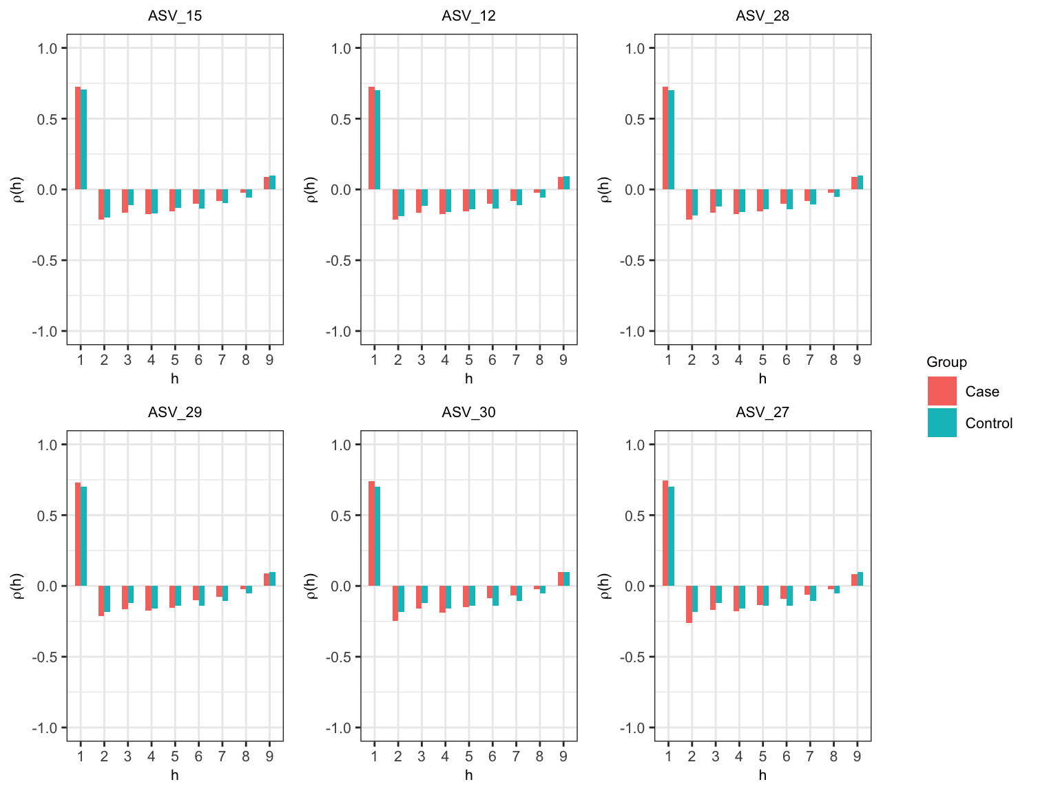
Partial autocorrelation within subject
Figure @ref(fig:pacf) shows that the largest spike (\(\left|\rho\left(h\right) \right| > .25\)) is observed at \(h = 1\) for both case and control in all ASVs. The spike at \(h = 2\) is closer to .25 for ASV_30 and ASV_27 in case. The spike decreases at \(h = 3\) and then, increases at \(h = 4\) for all ASVs. Thus, We can assume that five consecutive observations make a block. We will choose an inital block size of 5 (\(l_{I} = 5.\)).
longitudinal data lag-plots
We can also check the lag-plot for each ASV. The interpretaion of lag plot is as follows:
- For each ASV, we plot arcsinh transformation values at different lags. The lag-plot is interpreted as follows:
- lack of autocorrelation is implied by the absence of a pattern in the lag plot,
- weak to moderate autocorrelation is implied by less clustering of points along the diagonal, and
- high autocorrelation is implied by tight clustering of points along the diagonal.
Let us check the lag-plot for ASV_30 at lags \(1, \cdots, 8\). We need to specify the ASV index in the ‘taxon’ option. In this example, ‘taxon = 30’.
lags <- as.list(seq(1, 8))

p.lags <- lapply(lags,function(x){
    longLagPlot(ps.tr,
        main_factor = "Group",
        time_var = "Time",
        taxon = 30,
        x,
        taxlevel = "Genus")})

#   Change the legend labels
p.lags <- lapply(p.lags, function(x){
    x + scale_color_discrete(name  = "Group",
      breaks = c("Case", "Control"),
      labels = c("Case", "Control"))
    })

leg <- plot_common_legend(p.lags[[1]])

plist <- lapply(p.lags,function(x){
    x+theme(legend.position = "none")
    })


# p <- grid.arrange(arrangeGrob(grobs=plist,nrow=2,widths=c(3,3,3,3)),
#                   leg,
#                   ncol=2,
#                   widths=c(10,2))
# fileN <- paste0("lag_plot_", setting_name, ".eps")
# ggsave(fileN, plot = p, width = 8, height = 5.5)

grid.arrange(arrangeGrob(grobs = plist,
  nrow = 2,
  widths = c(3, 3, 3, 3)),
  leg,
  ncol = 2, widths = c(10, 2),
  top = textGrob("ASV 30",
    gp = gpar(fontsize = 8, font = 3)))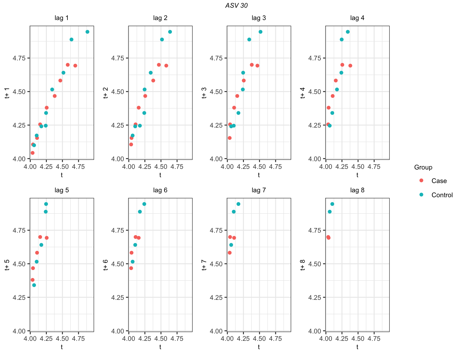
Lag-plot for ASV_30
Figure @ref(fig:lag-plots) shows that (for ASV 30) that points are almost on the diagonal at \(h = 1\). Then, points are less clustering along the diagonal at \(h = 3\). We can either choose an initial block size of 4 according to lag-plot or 5 accroding to PACF. However, we visualized a lag-plot for one ASV but we visualized PAC for six ASVs. Thus, we will still choose \(l_{I} = 5.\)
In practice, we can choose initial block size using PAC plots. If there are spurious effects at larger lags and suggesting to choose BIG initial block size, we can diagnose those using lag-plot for particular ASV. There might be a spurious higher autocorrelation at larger lags due to a small number of observations or abundances close to zero.
Correlogram
In practice, we can also choose \(l_{I}\) using correlogram. First, we use the variance-stabilizing transformation on the original abundance table. Then, for each ASV, we compute the average transformed abundance at each time point. Finally, we plot within-subject autocorrelation for top six abundances ASVs. These top six ASVs are selected according to the sum of transformation values for each ASV. Using the autocorrelation plots, we consider the first occurrence of a lag with sufficiently close to zero autocorrelation as initial block size \(l_{I}\). There might be a spurious higher autocorrelation at larger lags due to a small number of observations or abundances close to zero.
p.all <- longCorreloMultiple(ps.tr,
  main_factor = "Group",
  time_var = "Time",
  starttaxa = 1,
  endtaxa = 6,
  taxlevel = "Genus")

#   Change the legend labels
p.all <- lapply(p.all, function(x){
    x + scale_fill_discrete(name  ="Group",
      breaks=c("Case", "Control"),
      labels=c("Case", "Control"))
    })

#   extract the common legend for all taxa
leg <- plot_common_legend(p.all[[1]])

plist <- lapply(p.all,function(x){
    x + theme(legend.position = "none")
    })

# p <- grid.arrange(arrangeGrob(grobs=plist,nrow=2,widths=c(3,3,3)),
#                   leg,
#                   ncol=2,
#                   widths=c(10,2))

# fileN <- paste0("correlogram_", setting_name, ".eps")
# ggsave(fileN, plot = p, width = 8, height = 5.5)
#
grid.arrange(arrangeGrob(grobs = plist,
  nrow = 2,
  widths = c(3, 3, 3)),
  leg,
  ncol = 2,
  widths=c(10, 2))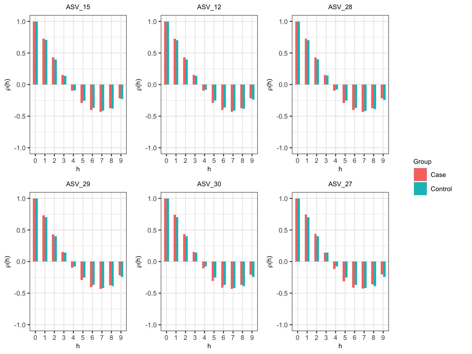
Correlogram
In Figure @ref(fig:corr) we observe that the correlogram tends to be sufficiently zero at \(h = 4\) for almost all the ASVs. Therefore, the initial block size is 5.
All exploratory tools suggest an inital block size of 5.
Now we have chosen the initial parameters for the subsampling method. \(\omega = .6\) and \(l_{I} = 5\).
The block bootstrap method
First, we identify the opitmal block size for the subsample. We use \(l_{I} = 5\) and subsampling proportion \(\omega = .6\) to identify the opitmal block size.
Subsampling
- Compute \(\psi(q, l_{I})\) and \(T_{i}\left(q, l_{I}\right)\) using the initial block size and the full data.
#####Note: With 4 cores, this will take almost 18 hours
R <- 200
RR <- 50
main_factor <- "Group"
time_var <- "Time"
subjectID_var = "SubjectID"
sampleID_var = "SampleID"
lI <- 5
omega <- .6

system.time(
    mse.results <- bootLongSubsampling(ps = ps,
        main_factor = main_factor,
        time_var = time_var,
        subjectID_var = subjectID_var,
        sampleID_var = sampleID_var,
        lI = lI,
        R = R,
        RR = RR,
        omega = omega,
        lC1 = lC1, lC2 = lC2,
        ncores = ncores,
      psi.hat.lI = FALSE,
      psi.hat.lI.val = NULL,
      compStatParallel = FALSE)
)

fileN <- paste0("./psi.hat.lI_", setting_name,".rds")
saveRDS(mse.results, fileN) - We can run the following code parallel for each block sizes (lC1 = lC2) if we have already saved
psi.hat.lI.- Save the mse results for each lC1
Use compStatParallel = TRUE if you have more ASVs than R.
##### NOTE: With 4 cores, this will take almost 71 hours

# fileN <- paste0("ps", setting_name, ".rds")
# ps <- readRDS(fileN)

fileN <- paste0("./psi.hat.lI_", setting_name,".rds")
psi.hat.lI.val <- readRDS(fileN)

R <- 200
RR <- 50
main_factor <- "Group"
time_var <- "Time"
subjectID_var = "SubjectID"
sampleID_var = "SampleID"
lI <- 5
omega <- .6

system.time(
    mse.results <- bootLongSubsampling(ps = ps,
        main_factor = main_factor,
        time_var = time_var,
        subjectID_var = subjectID_var,
        sampleID_var = sampleID_var,
        lI = lI,
        R = R,
        RR = RR,
        omega = omega,
        lC1 = lC1, lC2 = lC2,
        ncores = ncores, psi.hat.lI = TRUE, psi.hat.lI.val = psi.hat.lI.val, compStatParallel = FALSE)
)

fileN <- paste0("MSE_", setting_name, "_lC1", lC1,".rds")
saveRDS(mse.results, fileN)
Inspect MSE plot
We combine the results for all the possible \(lC1\). In this example, \(lC1 = 2, 3, 4\)
MSE.all <- list()
for(lC1 in 2:4){
  filename <- paste0("MSE_",setting_name,"_lC1", lC1,".rds")
  MSE.all[(lC1-1)] <- readRDS(filename)
}

fileN <- paste0("MSE_",setting_name,".rds")
saveRDS(MSE.all, fileN)
Find the optimal block size for the subsample (l_{}) using MSE plot.
Find the optimal block size for the original data using the formula.
\[l_{o} = \left(\frac{1}{\omega}\right)^{1/5}l_{\omega}\].
lC1 <- 2
omega <- .6
fileN <- paste0("MSE_",setting_name,".rds")
mse.results <- readRDS(fileN)

blks <- length(mse.results)
mse <- list()

for(i in 1:blks){
    mse[[i]] <- mse.results[[i]]$MSE_i
    }

mse.avg <- lapply(mse,function(x){mean(x, na.rm=T)})
mse.sum <- lapply(mse,function(x){sum(x, na.rm=T)})

mse <- unlist(mse.sum)
lblk <- seq(lC1, (length(mse)+1), by=1)
lblk.f <- as.factor(lblk)
dfp <- data.frame(mse = mse,lblk = lblk.f)

l.omega <- lblk[mse==min(mse)]
l.omega
l.opt <- round((100/(omega*100))^(1/5)*l.omega, digits = 0)
l.opt

p.mse <- ggplot(dfp, aes(x=lblk, y=mse, group=1))+
    geom_point()+
    geom_line()+
    xlab("block size")+
    ylab("Mean squared error")+
    ggtitle(paste0("MSE for  ", setting_name, " ", omega*100,"%"," subsample")) +
  theme(plot.title = element_text(hjust = 0.5))

p.mse

fileN <- paste0("MSE_", setting_name, ".eps")
ggsave(fileN, plot = p.mse, width = 8, height = 5.5)
Run the block bootstrap method with the optimal block size \(l_{o}\)
Finally, we run the block bootstrap method with the optimal block size for differential abundance analysis.
#### Note: With 4 cores, this will take 17 hours
R <- 200
RR <- 50
main_factor <- "Group"
time_var <- "Time"
subjectID_var = "SubjectID"
sampleID_var = "SampleID"

sample_data(ps)$Group <- factor(sample_data(ps)$Group)
sample_data(ps)$Group <- relevel(sample_data(ps)$Group, ref = "Control")

system.time(
    MBB.all <- bootLongMethod(ps,
        main_factor = main_factor,
        time_var = time_var,
        sampleID_var = sampleID_var,
        subjectID_var = subjectID_var,
        b = l.opt,
        R = R,
        RR = RR, FDR = .05, compStatParallel = FALSE)
    )

fileN <- paste0("MBB_",setting_name,".rds")
saveRDS(MBB.all, fileN)
Inspect the MBB results
We can make a summary of differential abundance ASV.
fileN <- paste0("ps", setting_name, ".rds")
ps <- readRDS(fileN)

FDR <- .05
taxalevel <- "Genus"

fileN <- paste0("MBB_",setting_name,".rds")
boot.res.all <- readRDS(fileN) # list("summary", "beta.hat", "beta.hat.star", "beta.hat.star.star", "T.obs")

summ <- boot.res.all$summary

### add strain number to interested taxonomy same as in EDA
tax_table(ps)[, taxalevel] <- paste0(tax_table(ps)[, taxalevel],"_st_",seq(1, ntaxa(ps)))

### if we change FDR, wee need to adjust the confidence interval
T.stars.and.obs <- boot.res.all$beta.hat.star

lcl <- apply(T.stars.and.obs, 1, FUN=function(x){
  quantile(x, probs=FDR/2, na.rm=TRUE)
  })
ucl <- apply(T.stars.and.obs, 1, FUN=function(x){
  quantile(x, probs=(1-FDR/2), na.rm=TRUE)
  })

summ$lcl <- lcl
summ$ucl <- ucl

summ.filt.FDR <- dplyr::filter(summ, pvalue.adj <= FDR)
summ.filt.FDR <- dplyr::select(summ.filt.FDR, one_of("ASV","stat","pvalue.adj","lcl","ucl"))
summ.filt.FDR <- dplyr::filter(summ.filt.FDR, !is.na(pvalue.adj))
summ.filt.FDR <- dplyr::arrange(summ.filt.FDR, desc(stat))

### To save the results
summ.filt.FDR$stat <- round(summ.filt.FDR$stat, digits = 2)
summ.filt.FDR$pvalue.adj <- round(summ.filt.FDR$pvalue.adj, digits = 4)
summ.filt.FDR$pvalue.adj[which(summ.filt.FDR$pvalue.adj==0)] <- "<.0001"
summ.filt.FDR$lcl <- round(summ.filt.FDR$lcl, digits = 2)
summ.filt.FDR$ucl <- round(summ.filt.FDR$ucl, digits = 2)

df.mbb <- data.frame(Taxa = summ.filt.FDR$ASV, betahat = summ.filt.FDR$stat, lcl = summ.filt.FDR$lcl, ucl = summ.filt.FDR$ucl, p.adj = summ.filt.FDR$pvalue.adj)

df.mbb.write <- df.mbb
df.mbb.write$Taxa <- tax_table(ps)[as.character(df.mbb.write$Taxa), taxalevel] %>% as.character

####if you would like to avoid completely the ASV with strain number only.

# is.it.st <- lapply(df.mbb.write$Taxa, function(x){(strsplit(x, "_") %>% unlist)[1]}) %>% unlist
# is.it.ind <- which(is.it.st == "st")
# df.mbb.write <- df.mbb.write[-is.it.ind, ]

library(xtable)
fileN <- paste0("MBB_",setting_name,".tex")
print(xtable(df.mbb.write, type = "latex", digits = c(0,0,2,2,2,4)), file = fileN)
Plot significant ASVs
####if you would like to avoid completely the ASV with strain number only.
#df.mbb <- df.mbb[-is.it.ind, ]
#
df.mbb <- dplyr::filter(df.mbb, abs(beta) > 1)
ps.tr <- psTransform(ps, main_factor = "Group")[[1]]

taxaName <-  tax_table(ps.tr)[, taxalevel] %>% as.character
ind <- which(taxa_names(ps) %in% as.character(df.mbb$Taxa))
tax.plot <- taxa_names(ps.tr)[ind]


otu.df <- otu_table(ps.tr) %>% t %>% data.frame
samdf <-  sample_data(ps.tr) %>% data.frame
otu.df <- bind_cols(otu.df, samdf)
colnames(otu.df)[1:ntaxa(ps.tr)] <- taxa_names(ps.tr)

otu.df.l <- gather(otu.df, key=taxa, value=abund, 1:ntaxa(ps.tr))
otu.df.l$taxa <- otu.df.l$taxa %>% factor
otu.df.l$Time <- otu.df.l$Time %>% factor

otu.df.l <- filter(otu.df.l,taxa %in% tax.plot)
otu.df.l$taxa <- droplevels(otu.df.l$taxa)

txname <- taxaName[ind]

match.tax.name <- data.frame(taxa = tax.plot, nam = txname)
rownames(match.tax.name) <- as.character(match.tax.name$taxa)
repl.tax.n <- match.tax.name[levels(otu.df.l$taxa),"nam"]

otu.df.l$taxa <- factor(otu.df.l$taxa,labels  = as.character(repl.tax.n))

otu.df.l$Time <- as.numeric(otu.df.l$Time)

p <- ggplot(otu.df.l)+
    geom_line(aes(x = Time, y = abund, linetype = Group, col = SubjectID, group = SubjectID))+
    facet_wrap(~taxa,scales = "fixed")+
    ylab("asinh")+
  xlab("Gestational Week") +
  ggtitle(paste0("Differentially Abundant Taxa (MBB) in ", setting_name)) +
    theme(strip.text.x = element_text(size = 10, face="italic", margin = margin(.1, 0, .05, 0, "cm")), axis.text=element_text(size=8, face = "bold"), plot.title = element_text(hjust = 0.5)) + scale_color_discrete(guide = FALSE) +
  scale_linetype_discrete(name  ="",breaks=c("Control", "Case"),labels=c("Control", "Case")) +
  stat_summary(aes(x = Time,y = abund, linetype= Group),fun.y = mean, geom = "line")

p

fileN <- paste0("Inspect_diff_abun_", setting_name, ".eps")
ggsave(fileN, plot=p, width = 12, height = 8)