Introduction

Characterizing the tumor ecosystem in breast cancer patients is vital for identifying prognosis and treatment. Single-cell targeted proteomics methods can quantify protein expression in tumor and immune cells and spatial coordinates of cells. However, the tumor ecosystem is phenotypically and functionally heterogeneous. Thus, we need to consider multiple targeted proteomics methods to deepen our understanding of the breast cancer tumor ecosystem.

We propose Bayesian latent Dirichlet allocation to jointly integrate two targeted proteomics data from different breast cancer patients with partially-overlapping proteomic markers. We then use samples drawn from the posterior to infer cell co-location based on the latent topic proportions in cells. We also infer the spatial location of CyTOF cells using the MIBI-TOF.

We illustrated the techniques using the mass cytometry (CyTOF) data of Wagner et al. (2019) and multiplexed ion beam imaging- time of flight (MIBI - TOF) data of Keren et al. (2018), studies on the tumor and immune ecosystem of human breast cancer patients. This vignette provides R scripts for the analysis.

Method

We extend MultiAssayExperiment Ramos et al. (2017) class to integrate multiple single-cell proteomics data. This container can be used for preprocessing, transformation, extracting spatial information from raster objects, and adding cell information, topic modeling, and visualization.

Keren et al. (2018) MIBI-TOF data are the size-normalized raw intensity values, arcsinh transformed and standardized across the markers. The distribution of transformed values shows that there are outliers in 32 protein markers. Wagner et al. (2019) CyTOF data are arcsinh transformed of intensity values. We do the inverse transformation of CyTOF data. We then use the upper limit of CyTOF data to scale the MIBI-TOF (normalized) data to the range of CyTOF data. After making the same units in both CyTOF and MIBI-TOF, we impute the protein expression that is not measured in one of the platforms using the nearest neighbor averaging Hastie et al. (2019). We round the protein expression to an integer.

We use topic modeling to find the dominated topics in CyTOF and MIBI-TOF cells Blei, Ng, and Jordan (2003). We assign the spatial location of MIBI-TOF cells to the CyTOF data based on the topic distribution in each cell (if the difference between the topic distribution of the dominated topic in the CyTOF and the dominated topic in the MIBI-TOF is the minimum.) We infer the spatial location of CyTOF cells using the MIBI-TOF (one patient, but we can increase the number of patients). We plot the spatial co-location of CyTOF cells related to the MIBI-TOF spatial location.

We use fitted topic modeling to simulate data that gives us the predicted value for MIBI-TOF markers that are not observed.

Results

Subject selection

We choose one patient from CyTOF (Live cells: immune panel) and one patient from MIBI-TOF, but the ideal is to use MIBI-TOF data from the same patient. For the topic modeling, we keep 10% cells from MIBI-TOF for the test data to choose an optimal number of topics as five $\left(K=5\right)$ based on the posterior log-likelihood.

K <- 5
K
iter <- 2000
iter

We load the required packages for the analysis.

library(SingleCellExperiment)
library(ggplot2)
library(rstan)
library(plyr)
library(reshape2)
library(readr)
library(magrittr)
library(MultiAssayExperiment)
library(dplyr)
library(DESeq2)
library(abind)
library(tibble)
library(RColorBrewer)
library(raster)
library(stringr)
library(ggthemes)
library(pheatmap)
library(gtools)
library(uwot)
library(gridExtra)

Data

Wagner 2018 Cytof
- 140 breast cancer patients; Of 140, 6 triple negative (TN)
- cd45_sce_dropna$Clinical.Subtype == "TN
- 3 cancer-free
- 73 protein markers in immune-centric and tumor-centric microenvironment
Keren 2018 Multiplex Ion Bean Imaging (MIBI-TOF)
- Tumor-immune microenvironment in TN patients
- 41 TN patients
- 36 proteins

Note: To create MultiAssayExperiment, we choose patients with TN with immune and tumor cells in both CyTOF and MIBI-TOF. Then, we select one patient from each CyTOF and MIBI-TOF for the integrative analysis.

Mass-Tag CyTOF Breast Cancer Data

We use cd45.sce: CD45+ cells from the live cells; down-sampled to 426,872 cells (assayed on immune panel) $\times$ 35 proteins.

load("masstagSCE.rda")
cd45.sce # 38 * 426872
rm(epith.sce, livecells.sce, myeloid.sce, tcell.sce)

We drop the five patients without any clinical data. We can use the Gender variable to identify those patients.

unique(colData(cd45.sce)$patient_id.y[which(is.na(colData(cd45.sce)$Gender))])

cd45_to_keep <- which(!is.na(colData(cd45.sce)$Gender))
cd45.sce_dropna <- cd45.sce[,cd45_to_keep]
cd45.sce_dropna # 38 * 420685
# To verify there are no (true) NA's left:
sum(is.na(rowData(cd45.sce_dropna)))
rm(cd45.sce, cd45_to_keep)

saveRDS(cd45.sce_dropna, "cd45_sce_dropna.rds")

cd45_sce <- readRDS("cd45_sce_dropna.rds")
cd45_sce

There are three proteins without gene symbol in cd45_sce_dropna, so we drop them (non-protein channels for cisplatin and DNA tags included.)

cd45_sce <- cd45_sce[!(rowData(cd45_sce)$hgnc_symbol == "na") ,]
cd45_sce

There are two different health status.

table(colData(cd45_sce)$Health.Status)

There are five different clinical subtypes of cancer patients, including TN and healthy.

table(colData(cd45_sce)$Clinical.Subtype)

We subset TN clinical subtype.

cd45_sce <- cd45_sce[, cd45_sce$Clinical.Subtype == "TN"]
cd45_sce
#drop cells(columns) with no protein expression
cd45_sce <- cd45_sce[, colSums(assay(cd45_sce)) > 0]
cd45_sce
# drop levels of patient_id.x
cd45_sce$patient_id.x <- droplevels(cd45_sce$patient_id.x)

There are six TN patients, and among them, two had previous cancer incidence.

table(cd45_sce$Previous.Cancer.Incidences, cd45_sce$patient_id.x)

We choose patient BB028 and infer the co-location of immune cells in the CyTOF data using MIBI-TOF data.

cd45_sce <- cd45_sce[ , cd45_sce$patient_id.x == "BB028"]
cd45_sce

We add cell ids to CyTOF.

cd45_sce$cell_id <- paste0("cytof_", seq(1, dim(cd45_sce)[2]))
colnames(cd45_sce) <- cd45_sce$cell_id

Heatmap of the protein expression in each cell of patient BB028.

or <- order(rowMeans(assay(cd45_sce)), decreasing=TRUE)
ass <- assay(cd45_sce)[or, ]

df <- as.data.frame(colData(cd45_sce)[colnames(ass), c("patient_id.x", "Menopause.Status", "Previous.Cancer.Incidences", "HER2.IHC.Score" ,"cell_id")])

df <- with(df, df[order(patient_id.x, Menopause.Status, Previous.Cancer.Incidences, HER2.IHC.Score, cell_id),])
ass <- ass[, df$cell_id]
df <- dplyr::select(df, -cell_id)

rownames(ass) <- rowData(cd45_sce)$marker_name[or]

p <- pheatmap(ass,
              annotation_col = df,
              cluster_rows = FALSE,
              cluster_cols = FALSE,
              fontsize_row = 14,
              fontsize_col = 14,
              show_colnames = FALSE)

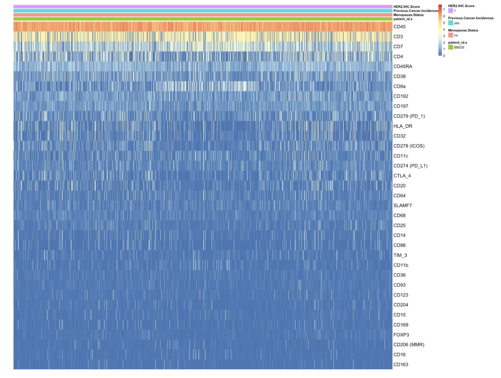
Heatmap of the protein expression in each cell of patient BB028.

Keren et al., MIBI-TOF Breast Cancer Data

All 39 patients were TN
The size-normalized raw intensity values are then arcsinh transformed and standardized across the markers.

load('mibiSCE.rda')
mibi.sce

summary(as.vector(assay(mibi.sce)))
rowMeans(assay(mibi.sce))
rowSds(assay(mibi.sce))
rowMax(assay(mibi.sce))

Rows correspond to channels, and columns correspond to cells. We can see all of the channels that were collected in this experiment.

rownames(mibi.sce)

The 38 proteins can be easily identified by using the binary attribute is_protein from rowData (The other 11 comprise background, experimental controls (e.g., Au and dsDNA), and elements of potential interest in studying cellular mechanisms (e.g., Ca, Fe; relevant in other spatial studies.)

mibi.sce_proteins <- mibi.sce[rowData(mibi.sce)$is_protein == 1,]
mibi.sce_proteins
rm(mibi.sce)

summary(as.vector(assay(mibi.sce_proteins)))
rowMeans(assay(mibi.sce_proteins))
rowSds(assay(mibi.sce_proteins))
rowMax(assay(mibi.sce_proteins))

Cell type information is available in the columns tumor_group and immune_group. That is, 51% of cells were Keratin positive tumor cells, and 41% of cells were immune cells.

round(table(mibi.sce_proteins$tumor_group)/ncol(mibi.sce_proteins),2)

Among the immune cells, macrophages, and CD8, CD4+ T-cells and other immune cells were identified. 10% of all cells assayed were macrophages.

# Immune Cells
round(table(mibi.sce_proteins$immune_group)/ncol(mibi.sce_proteins),2)

We consider Keratin positive tumor cells and immune cells (there are different immune cell types within immune cells.)

table(colData(mibi.sce_proteins)$tumor_group)
table(colData(mibi.sce_proteins)$tumor_group, colData(mibi.sce_proteins)$immune_group)

mibi.sce_proteins <- mibi.sce_proteins[, colData(mibi.sce_proteins)$tumor_group %in% c("Immune", "Keratin-positive tumor")]

mibi <- mibi.sce_proteins
mibi
#drop cells(columns) with no protein expression
mibi <- mibi[, colSums(assay(mibi)) > 0]
mibi
#drop proteins(rows) with no expression in any of these cells
mibi <- mibi[rowSums(assay(mibi)) > 0, ]
mibi

rowData(mibi) does not have cell IDs, so we add it.

colData(mibi)$cell_id <- paste0("mibi_", seq(1, dim(mibi)[2]))
colnames(mibi) <- colData(mibi)$cell_id
mibi$DONOR_NO <- mibi$DONOR_NO %>% as.character()

There are mibi$SampleID 42, 43, 44 with no DONOR_NO, and we remove cells from these SampleIDs.

mibi <- mibi[, !(mibi$SampleID %in% c("42", "43", "44"))]
mibi

Heatmap of protein expression in tumor and immune cells (50 randomly selected) in randomly selected five patients in MIBI-TOF data.

or <- order(rowMeans(assay(mibi)), decreasing=TRUE)

g <- mibi$DONOR_NO %>% factor()
choose_by_patient <- split(colData(mibi)%>% data.frame, g)
sample_by_patient <- sample(seq(1, length(choose_by_patient)), 5)


no_cells_per_patient <- table(mibi$DONOR_NO) %>% data.frame()
no_cells_per_patient <- data.frame(no_cells_per_patient$Freq)
no_cells_sample <- apply(no_cells_per_patient, 1, function(y){
  min(50, y)
})

patient_list <- as.list(seq(1, length(choose_by_patient)))

choose_by_patient_cells <- lapply(patient_list, function(x){
  sample_cell_ids <- sample(choose_by_patient[[x]]$cell_id, no_cells_sample[x])

  return(sample_cell_ids)

})
choose_by_patient_cells <- choose_by_patient_cells[sample_by_patient]

choose_by_patient_cells <- choose_by_patient_cells %>% unlist()
names(choose_by_patient_cells) <- NULL

ass <- assay(mibi)[or, which(mibi$cell_id %in%  choose_by_patient_cells)]


df <- as.data.frame(colData(mibi)[colnames(ass), c("DONOR_NO", "tumor_group", "immune_group","cell_id")])

df <- with(df, df[order(DONOR_NO, tumor_group, immune_group,cell_id), ])
ass <- ass[, df$cell_id]
df <- dplyr::select(df, -cell_id)

rownames(ass) <- rownames(rowData(mibi))[or]

p <- pheatmap(ass,
              annotation_col = df,
              cluster_rows = FALSE,
              cluster_cols = FALSE,
              fontsize_row = 14,
              fontsize_col = 14,
              show_colnames = FALSE)

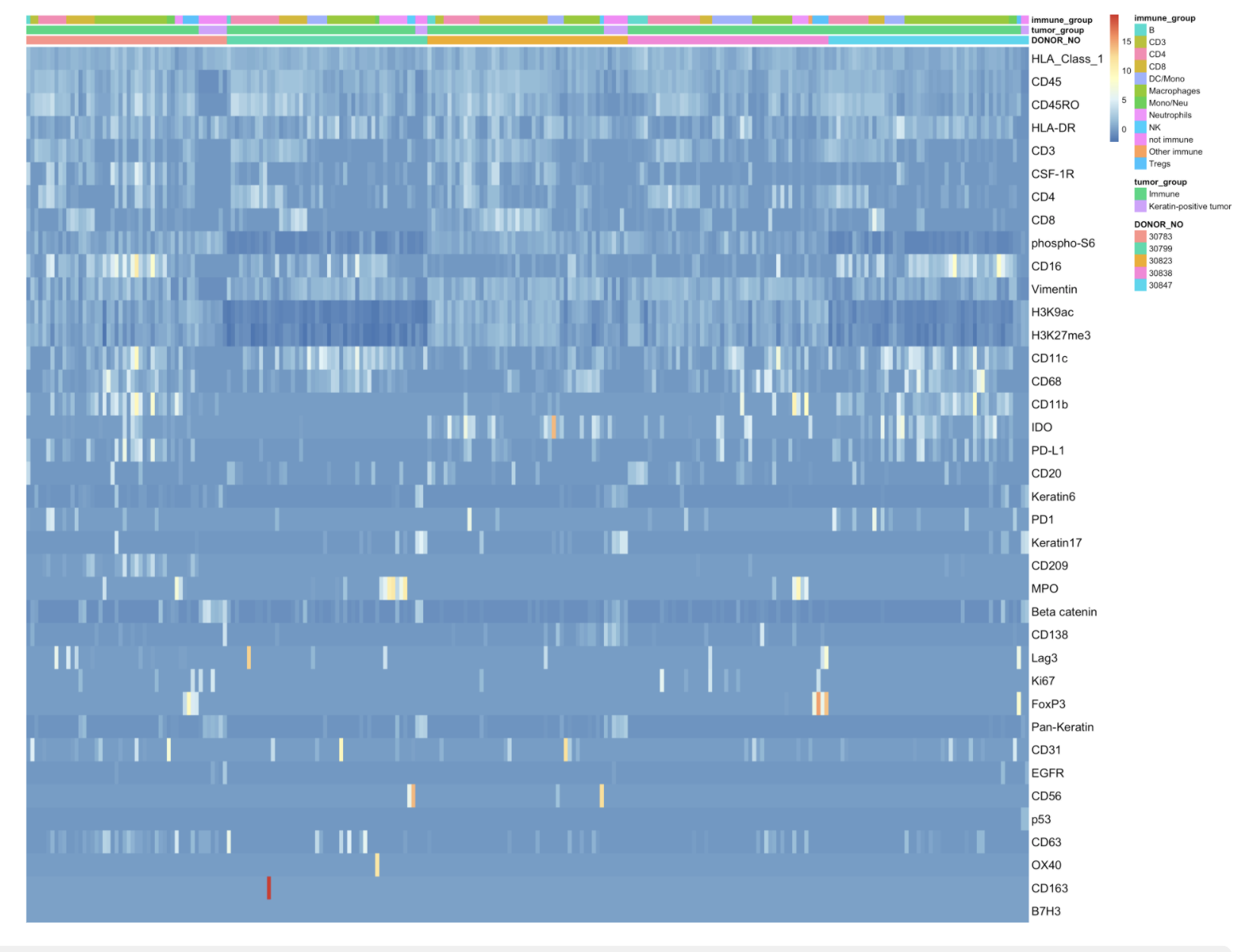
Heatmap of protein expression in tumor and immune cells in randomly selected five patients in MIBI-TOF data.

cell_type <- ifelse(mibi$immune_group != "not immune", mibi$immune_group, "Tumor")
mibi$cell_type <- cell_type

Spatial information

Because we already run this code, we read the saved mae (MultiAssayExperiment) with spatial information.

tiff_file_list <- list.files("TNBC_shareCellData/", pattern = ".tiff")

mibi_sample_id_list <- list()
for(id in 1:length(tiff_file_list)){
    str_name <- paste("TNBC_shareCellData/", tiff_file_list[id], sep = "")

    sample_id <- as.numeric(gsub("p", "", gsub("_labeledcellData.tiff", "", tiff_file_list[id])))

    r <- raster(str_name)

    mibi_sample_id_list[[id]] <- mibi[, mibi$SampleID == sample_id]

    df_rP <- rasterToPoints(r)
    df_rP <- data.frame(df_rP)
    colnames(df_rP) <- c("X", "Y", "values")
    noise_not_in_mibi <- unique(df_rP$values[!df_rP$values %in% mibi_sample_id_list[[id]]$cellLabelInImage])

    # compute centroid of each cell
    centroid_X <- aggregate(df_rP[,1], by = list(df_rP[,3]), FUN = median)
    centroid_Y <- aggregate(df_rP[,2], by = list(df_rP[,3]), FUN = median)
    centroid_XY <- data.frame(centroid_X = centroid_X$x, centroid_Y = centroid_Y$x, group = centroid_X$Group.1)
    cell_label_with_bg_XY <- mapvalues((centroid_XY$group), from = noise_not_in_mibi, to = rep(0, length(noise_not_in_mibi)))

    cell_label_with_bg_XY <- mapvalues((cell_label_with_bg_XY), from = mibi_sample_id_list[[id]]$cellLabelInImage, to = mibi_sample_id_list[[id]]$cell_type)
    centroid_XY$cell_label_with_bg_XY <- cell_label_with_bg_XY

    # filter the center info without cells 
    centroid_XY <- centroid_XY[centroid_XY$cell_label_with_bg_XY != "0", ]


    dd_sample_id <- colData(mibi_sample_id_list[[id]]) %>% data.frame()
    dd_sample_id <- left_join(dd_sample_id, centroid_XY, by = c("cellLabelInImage" = "group"))
    mibi_sample_id_list[[id]]$centroid_X <- dd_sample_id$centroid_X
    mibi_sample_id_list[[id]]$centroid_Y <- dd_sample_id$centroid_Y
}

mibi_spa <- cbind(mibi_sample_id_list[[1]], mibi_sample_id_list[[2]])
for(id in 3:length(tiff_file_list)){

 mibi_spa <- cbind(mibi_spa, mibi_sample_id_list[[id]])
}

saveRDS(mibi_spa, file = paste0("../Results/mibi_spa.rds"))

mibi <- readRDS("mibi_spa.rds")

We choose one DONOR from MIBI-TOF data.

mibi <- mibi[, mibi$DONOR_NO %in% "30824"]
mibi

#drop proteins(rows) with no expression in any of these cells
mibi <- mibi[rowSums(assay(mibi)) > 0, ]
mibi

#drop proteins(rows) with no expression in any of these cells
cd45_sce <- cd45_sce[rowSums(assay(cd45_sce)) > 0, ]
cd45_sce

Multiplicative error due to different scales

cd45_sce asinh transformation with cofactor 5

inv_func <- function(x) {
  5*sinh(x)
}
cd45_sce_inv <- cd45_sce
rm(cd45_sce)
assay(cd45_sce_inv) <- inv_func(assay(cd45_sce_inv))

Converting each scale to have the same lower and upper levels

Let $y$ is the rescaled variable and $x$ is the observed variable. $y = \left(\dfrac{x-x_{\text{min}}}{x_{\text{range}}}\right) \times u$, where $u$ is the upper limit of the rescaled variable.

We scale CyTOF and MIBI-TOF to upper limit of CyTOF.

u <- max(assay(cd45_sce_inv))
x_mibi <- assay(mibi)
y_mibi <- apply(x_mibi, 1, function(x){
  xmin <- min(x)
  xrange <- max(x) - min(x)
  y <- (x-xmin)/xrange*u
  return(y)
})
y_mibi <- t(y_mibi)

assay(mibi) <- y_mibi

Merge two `SingleCellExperiment` objects and make `MultiAssayExperiment`

source("../R/makeMAEfromSCE.R")
mae <- makeMAEfromSCE(sce_list = list(cd45_sce_inv, mibi),
                      name_assays = c("cd45", "mibi"),
                      sampleID_name = "cell_ID")
mae

Join the assays and impute

We already run this code, so we read the imputed data.

x1 <- assay(mae[["cd45"]]) %>% t() %>% data.frame()
x2 <- assay(mae[["mibi"]]) %>% t() %>%  data.frame()
x <-  full_join(x1, x2)
markers <- colnames(x)
cells <- c(rownames(x1), rownames(x2))
common_markers <- colnames(x1)[colnames(x1) %in% colnames(x2)]
common_markers

# some features are not recorded in one domain - impute data after scaling
colMissing <- apply(x, 2, function(y){mean(is.na(y))})

temp <- x %>% as.matrix() %>% t()

imdata <- impute::impute.knn(temp, k=5, rowmax = 0.5, colmax = 0.9)$data # temp is variables in the rows and samples in the columns
# x[is.na(x)] <- 0
saveRDS(imdata, "imdata_mibi_cytof_one.rds")

imdata <- readRDS("imdata_mibi_cytof_one.rds")
x <- imdata %>% t()
rownames(x) <- cells

Topic modeling

Split train and test set

For the topic modeling, we keep 10% cells from MIBI-TOF for the test data to choose an optimal number of topics as five based on the posterior log-likelihood.

test_samples <- sample(rownames(x2), size = round(length(rownames(x2))*0.1, digits = 0))
saveRDS(test_samples, file = "test_samples_one_mibi_one_cytof.rds")

test_samples <- readRDS("test_samples_one_mibi_one_cytof.rds")
x_test_train <- x
x_test <- x[test_samples, ]
x_test <- apply(x_test , c(1,2), function(y){as.integer(y)})
x_test <- as.matrix(x_test)
mae_test <- mae[, test_samples,]

Train dataset

x_train <- x[!(rownames(x) %in% test_samples), ]
x_train <- apply(x_train , c(1,2), function(y){as.integer(y)})
x_train <- as.matrix(x_train)
mae_train <- mae[, which(!(rownames(x) %in% test_samples)),]

Input for topic model

$K$ number of topics, $V$ number of features, $D$ number of cells, $\alpha$ hyperparameter of Dirichlet distribution over topics, $\gamma$ hyperparameter of Dirichlet distribution over features in each topic.

We set 0.8 for $\alpha$ across all cells and 0.5 for $\beta_{t}, t = 1, 2, \cdots, T$ across all features.

# theta[d] ~ dirichlet(alpha), alpha pseudocount for each topic
# beta[k] ~ dirichlet(gamma), gamma pseudocount for each feature in each topic
stan.data <- list(K = K,
  V = ncol(x_train),
  D = nrow(x_train),
  n = x_train,
  alpha = rep(.8, K),
  gamma = rep(.5, ncol(x_train))
)

We run the topic model for different $K = 3, 4, 5, 15, 20$.

fileN <- paste0("LDA_mibi_cytof_one_K_",K,"_ite_",iter,".RData")
fileN

We estimate the parameters using HMC No-U-Turn Sampler (NUTS) with four chains and 2000 iterations. Out of these 2000 iterations, 1000 iterations are used as warm-up samples.

t1 <- proc.time()
stan.fit <- stan(file = "./lda.stan",
  data = stan.data,
  iter = iter,
  chains = 4,
  sample_file = NULL,
  diagnostic_file = NULL,
  cores = 4,
  control = list(adapt_delta = 0.9),
  save_dso = TRUE,
  algorithm = "NUTS")
proc.time() - t1

save(stan.fit, file = fileN)

load(file = fileN)

Sampler diagnostics:

sampler_params <- get_sampler_params(stan.fit,
                                     inc_warmup = FALSE)
colnames(sampler_params[[1]])

mean_accept_stat_by_chain <- sapply(sampler_params,
                                    function(x) mean(x[, "accept_stat__"]))
mean_accept_stat_by_chain

max_treedepth_by_chain <- sapply(sampler_params,
                                 function(x) max(x[, "treedepth__"]))
max_treedepth_by_chain

Visualization

Extract posterior samples

samples <- rstan::extract(stan.fit,
                          permuted = TRUE,
                          inc_warmup = FALSE,
                          include = TRUE)# samples is a list

Alignment

Due to the label-switching problem across chains, it is not possible directly computing conditional log posterior $\hat{R}$ (split), effective sample size for model assessment, and evaluating convergence and mixing of chains. To address this issue, we fix the order of topics in chain one and then find the permutation that aligns the topics across four chains. For each chain two to four, we identify the estimated topics pair with the highest correlation, then find the next highest pair among the remaining, and so forth.

source("../R/alignmentMatrixMAE.R")
source("../R/thetaAligned.R")
theta <- samples$theta
aligned <- alignmentMatrixMAE(theta,
                           mae_train,
                           K,
                           iter = iter,
                           chain = 4,
                           SampleID_name = "cell_id")
theta_aligned <- thetaAligned(theta,
                              K,
                              aligned,
                              iter = iter,
                              chain = 4)
dimnames(theta_aligned)[[2]] <- mae_train$cell_id
dimnames(theta_aligned)[[3]] <- c(paste0("Topic_", seq(1,K)))

# array to a dataframe
theta_all <- melt(theta_aligned)
colnames(theta_all) <- c("iteration", "Sample", "Topic", "topic.dis")
theta_all$Chain <- paste0("Chain ", rep(seq(1, 4), each = (iter/2)))

sam <- colData(mae_train) %>% data.frame()
theta_all$Sample <- as.character(theta_all$Sample)
theta_all <- left_join(theta_all, sam, by =c("Sample"= "cell_id"))
theta_all$Chain <- factor(theta_all$Chain)
theta_all$Topic <- factor(theta_all$Topic)
theta_all$Sample <- factor(theta_all$Sample)

theta_all$cell_type <- factor(theta_all$cell_type)
theta_all$method <- ifelse(is.na(theta_all$cell_type), "cytof", as.character(theta_all$cell_type))

manual_col <- tableau_color_pal("Classic 20")(length(unique(theta_all$method)))

theta_summary <- theta_all %>%
  group_by(Sample, Topic, method) %>%
  summarize(median.topic.dis = median(topic.dis)) %>%
  ungroup() %>%
  mutate(Topic = factor(Topic, levels = rev(str_c("Topic_",1:K))))

#theta_summary <- dplyr::filter(theta_summary, cell_type %in% c("Macrophages", "Tumor"))

sample_cells <- unique(theta_summary$Sample)
sample_cells_select <- sample(sample_cells, 100)

theta_summary <- dplyr::filter(theta_summary,
                               Sample %in% sample_cells_select)

p <- ggplot(theta_summary,
           aes(x = method,
               y = Topic,
               fill = method))
p <- p+
  geom_tile(aes(alpha = median.topic.dis))+
  facet_grid(.~Sample, scale = "free")+
  xlab("method") +
  scale_fill_manual(name = "method",
                    values = manual_col) +
  scale_alpha(name = "median topic distribution") +
  theme_minimal(base_size = 20) +
  theme(plot.title = element_text(hjust = 0.5),
        strip.text.x = element_text(angle = 90),
        axis.text.x=element_blank())
p

# ggsave(paste0("topic_dis_mibi_cytof_one_K_",K, ".png"), p, width = 20, height = 6)

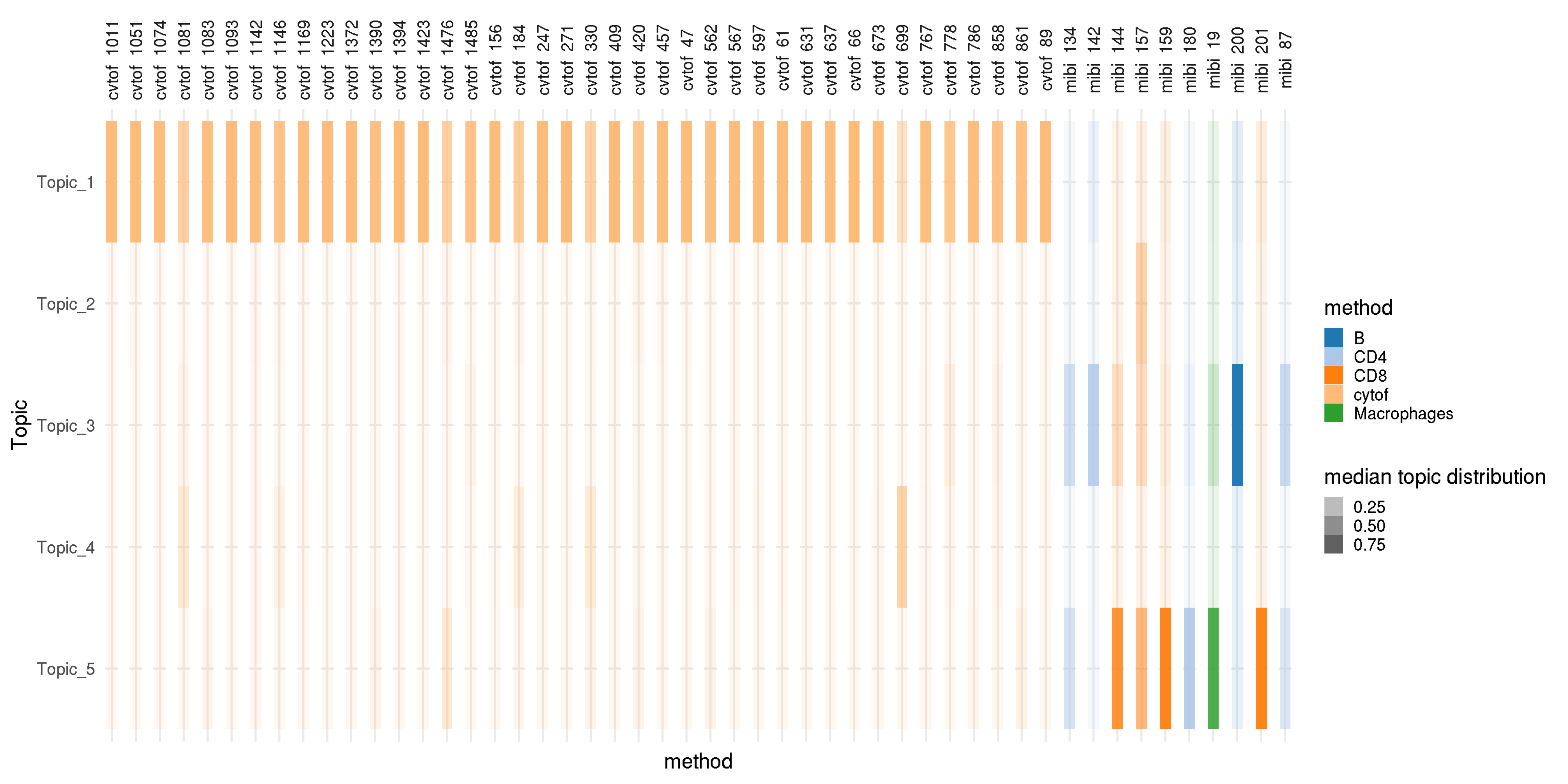
Topic distribution in each cell. With the five topics, the first topic is dominated in most of the immune cells from CyTOF data, and other topics are dominated in other cell types from MIBI-TOF data.

Feature distribution

source("../R/betaAligned.R")
beta <- samples$beta # an array (iterations *topic * marker)
beta_aligned <- betaAligned(beta,
                            K,
                            aligned,
                            iter = iter,
                            chain = 4) # an array (iterations *topic * ASV)

# array to data frame
beta_hat <- beta_aligned %>%
  melt(varnames = c("iterations", "topic", "marker_ix"),
       value.name = "beta_h") %>% as_tibble()
beta_hat$marker <- colnames(x_train)[beta_hat$marker_ix]


# join rowData with beta_hat
marker_info <- full_join(rowData(mae_train[["cd45"]]) %>% data.frame(), rowData(mae_train[["mibi"]]) %>% data.frame())
marker_info$marker <- marker_info$marker_name


beta_hat <- beta_hat %>%
  left_join(marker_info, by = "marker") %>% mutate(topic = paste("Topic", topic))


beta_hat$marker <- factor(beta_hat$marker)
beta_hat$marker_ix <- factor(beta_hat$marker_ix)
beta_hat$topic <- factor(beta_hat$topic)


beta_summary <- beta_hat %>%
  dplyr::group_by(marker_ix, topic) %>%
  dplyr::summarise(
    marker = marker[1],
    beta_median = median(beta_h),
    marker = marker[1],
    hgnc_symbol = hgnc_symbol[1]
  )

beta_subset <- beta_summary
beta_subset$marker_ix <- rep(seq_len(nrow(beta_subset) / K), each = K)

beta_subset <- beta_subset %>%
  arrange(marker_ix, topic)

beta_subset <- beta_subset %>%
  mutate(Class = factor(marker, levels = unique(beta_subset$marker)),
         Topic = str_remove(topic, "Topic "))


beta_subset$Topic <- factor(beta_subset$Topic, levels = seq(1,K) %>% as.character())

p <- ggplot(beta_subset,
            aes(x = Topic,
                y = marker,
                fill = beta_median)) +
  geom_tile() +
  ylab("Marker")+
  scale_fill_gradientn(name = "Median ASV distribution",
                       colours = c("gray98", "dodgerblue")) +
  theme_minimal(base_size = 20) +
  theme(plot.title = element_text(hjust = 0.5))

p
# ggsave(paste0("fea_dist_barplot_mibi_cytof_one_K_",K, ".png"), p, width = 13, height = 11)

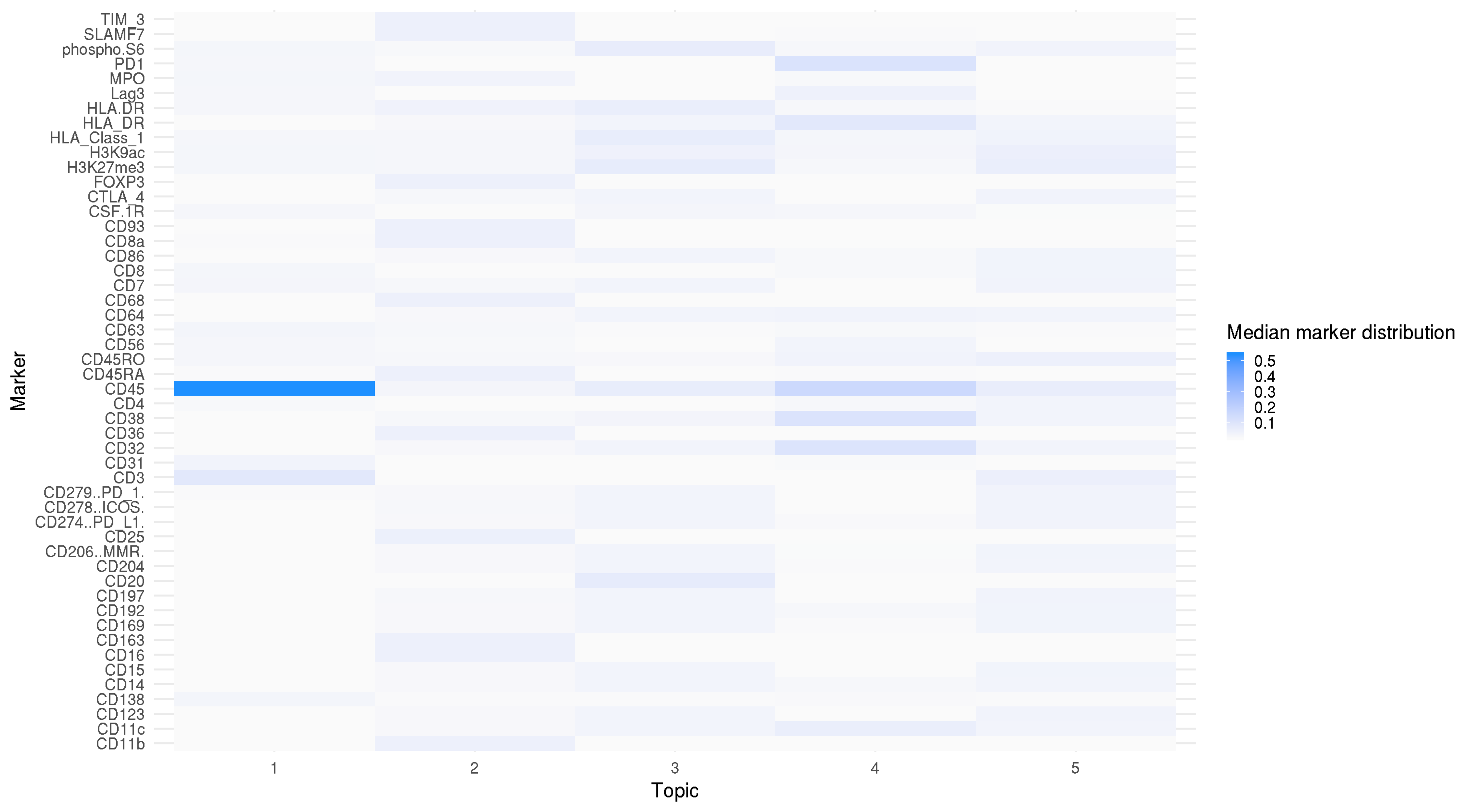
Marker distribution over topics. CD45 marker has the largest proportion in Topic 1.

The topic distribution shows that the first topic is dominated in most of the immune cells from CyTOF data; four other topics are dominated in all other cells. Feature distribution shows that cells from MIBI-TOF make five clusters consistently based on the observed and predicted marker expression, but these clusters are not identified with only observed marker expressions.

Computing statistics after alignment

Log posterior on the test data

We save posterior log-likelihood on test for different $K$ on test data.

dimnames(x_test) = NULL
test_data = list(K = K,
  V = ncol(x_test),
  D = nrow(x_test),
  n = x_test,
  alpha = rep(.8, K),
  gamma = rep(.5, ncol(x_test))
)

log_lik_total_for_each_iteration <- numeric()
for(it in 1:((iter/2)*4)){
  log_lik <- numeric()
    for(j in 1:dim(x_test)[1]){# For each sample j in the test set
      theta_aligned_sim <- rdirichlet(1, test_data$alpha)# simulate topic distribution from prior distribution
      p_vec_pos <- as.matrix(t(beta_aligned[it, , ])) %*% matrix(theta_aligned_sim, nrow = K, byrow = T)

      log_lik[j] <- dmultinom(x_test[j, ], size = sum(x_test[j, ]), prob = p_vec_pos, log = TRUE)
    }
  log_lik_total_for_each_iteration[it] <- sum(log_lik)
}


df_lp_corrected <- data.frame(lp = log_lik_total_for_each_iteration,
                             Chain = paste0("Chain ", rep(seq_len(4), each = (iter/2))))

fileN <- paste0("df_lp_test_mibi_cytof_one_K_", K, ".rds")
saveRDS(df_lp_corrected, fileN)

df_lp_corrected_all_K <- data.frame()
for(top in c(3:5, 15,20)){
  fileN <- paste0("df_lp_test_mibi_cytof_one_K_", top, ".rds")
  df_lp_corrected <- readRDS(fileN)
  df_lp_corrected$Num_Topic <- paste0("T=", rep(top, dim(df_lp_corrected)[1]))
  df_lp_corrected_all_K <- rbind(df_lp_corrected_all_K, df_lp_corrected)
}

df_lp_corrected_all_K$Num_Topic <- factor(df_lp_corrected_all_K$Num_Topic, levels = c(paste0("T=", c(seq(3, 5), 15, 20))
))

p <- ggplot(data = df_lp_corrected_all_K) +
  geom_boxplot(aes(x = Num_Topic, y = lp)) +
  ylab("Predictive log-likelihood in test data") +
  xlab("Number of topics")

p
# ggsave("lp_test_mibi_cytof_one.png", p, width = 7, height = 4)

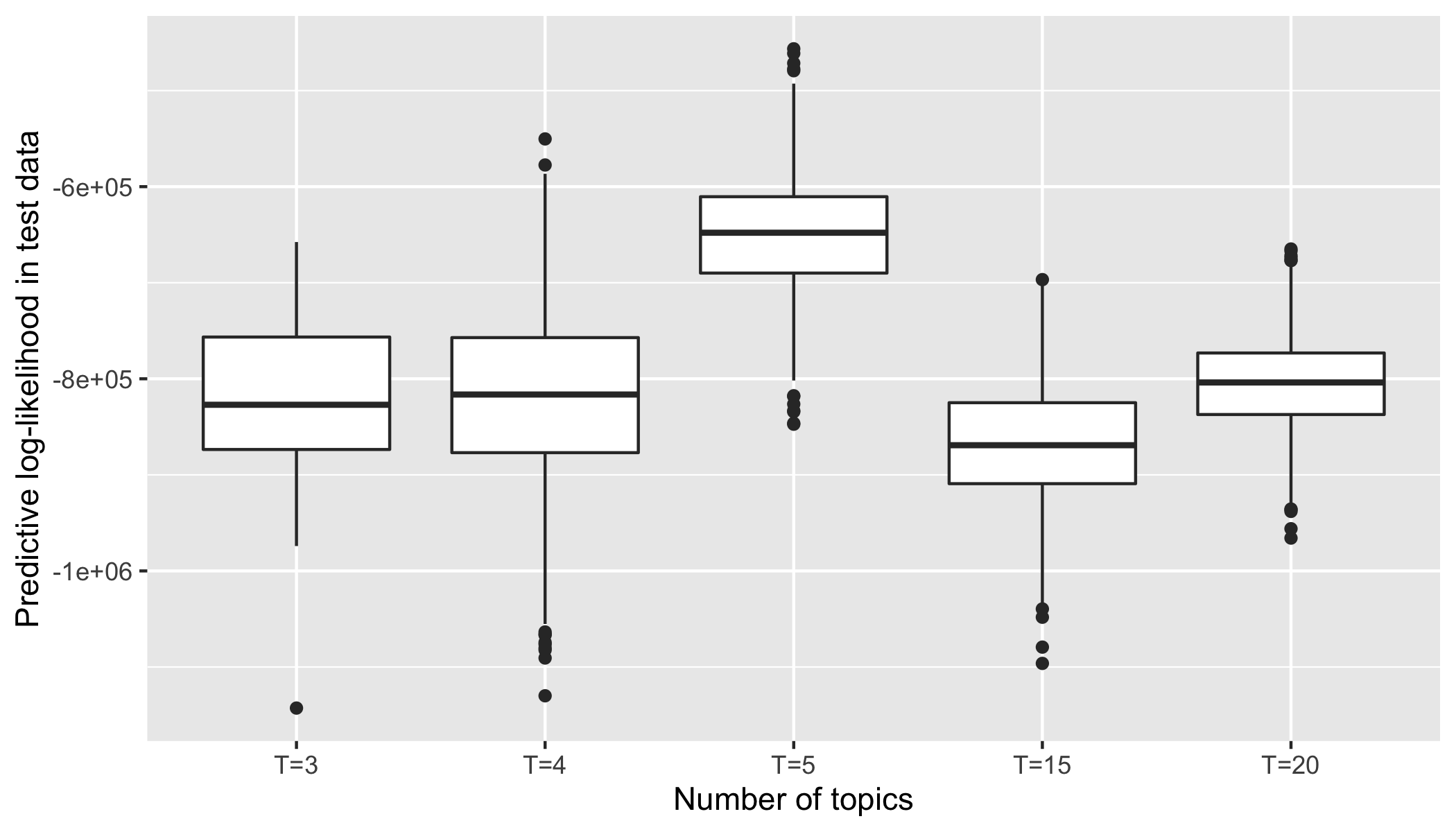
Posterior log-likelihood on test data.

Convergence diagnostics

Compute $\hat{R}$.

Rhat_theta <- matrix(nrow = dim(theta_aligned)[2], ncol = dim(theta_aligned)[3])
ESS_bulk_theta <- matrix(nrow = dim(theta_aligned)[2], ncol = dim(theta_aligned)[3])
ESS_tail_theta <- matrix(nrow = dim(theta_aligned)[2], ncol = dim(theta_aligned)[3])
for(sam in 1:dim(theta_aligned)[2]){
  for(top in 1:dim(theta_aligned)[3]){
    sims_theta <- matrix(theta_aligned[ ,sam , top], nrow = (iter/2), ncol = 4, byrow = FALSE)
    Rhat_theta[sam, top] <- Rhat(sims_theta)
    ESS_bulk_theta[sam, top] <- ess_bulk(sims_theta)
    ESS_tail_theta[sam, top] <- ess_tail(sims_theta)
  }

}

Rhat_theta <- as.vector(Rhat_theta)
ESS_bulk_theta <- as.vector(ESS_bulk_theta)
ESS_tail_theta <- as.vector(ESS_tail_theta)

Rhat_beta <- matrix(nrow = dim(beta_aligned)[2], ncol = dim(beta_aligned)[3])
ESS_bulk_beta <- matrix(nrow = dim(beta_aligned)[2], ncol = dim(beta_aligned)[3])
ESS_tail_beta <- matrix(nrow = dim(beta_aligned)[2], ncol = dim(beta_aligned)[3])

for(top in 1:dim(beta_aligned)[2]){
    for(fea in 1:dim(beta_aligned)[3]){
      sims_beta <- matrix(beta_aligned[ , top, fea], nrow = (iter/2), ncol = 4, byrow = FALSE)
      Rhat_beta[top, fea] <- Rhat(sims_beta)
      ESS_bulk_beta[top, fea] <- ess_bulk(sims_beta)
      ESS_tail_beta[top, fea] <- ess_tail(sims_beta)
    }

}

Rhat_beta <- as.vector(Rhat_beta)
ESS_bulk_beta <- as.vector(ESS_bulk_beta)
ESS_tail_beta <- as.vector(ESS_tail_beta)

Rhat <- c(Rhat_theta, Rhat_beta)
# fileN <- paste0("Rhat_mibi_cytof_one_K_",K, ".rds")
# saveRDS(Rhat, fileN)

ESS_bulk <- c(ESS_bulk_theta, ESS_bulk_beta)
# fileN <- paste0("ESS_bulk_mibi_cytof_one_K_",K, ".rds")
# saveRDS(ESS_bulk, fileN)

ESS_tail <- c(ESS_tail_theta, ESS_tail_beta)
# fileN <- paste0("ESS_tail_mibi_cytof_one_K_",K, ".rds")
# saveRDS(ESS_tail, fileN)

# R hat ~ 1.05
p_rhat <- ggplot(data.frame(Rhat = Rhat)) +
  geom_histogram(aes(x = Rhat),
                 fill = "lavender",
                 colour = "black",
                 bins = 100) +
  theme_minimal(base_size = 20) +
  theme(plot.title = element_text(hjust = 0.5))  +
  theme_minimal(base_size = 20) +
  xlab("")
p_rhat


# ggsave(paste0("/Rhat_mibi_cytof_one_K_",K, ".png"), p_rhat, width = 9, height = 6)

Compute ESS

# ESS bulk and ESS tail at least 100 per Markov Chain in order to be reliable and indicate that estimates of respective posterior quantiles are reliable

p_ess_bulk <- ggplot(data.frame(ESS_bulk = ESS_bulk)) +
  geom_histogram(aes(x = ESS_bulk),
                 fill = "lavender",
                 colour = "black",
                 bins = 100) +
  theme_minimal(base_size = 20) +
  theme(plot.title = element_text(hjust = 0.5))   +
  theme_minimal(base_size = 20) +
  xlab("")


p_ess_bulk

# ggsave(paste0("ess_bulk_mibi_cytof_one_K_",K, ".png"), p_ess_bulk, width = 9, height = 6)

p_ess_tail <- ggplot(data.frame(ESS_tail = ESS_tail)) +
  geom_histogram(aes(x = ESS_tail),
                 fill = "lavender",
                 colour = "black",
                 bins = 100) +
  theme_minimal(base_size = 20) +
  theme(plot.title = element_text(hjust = 0.5))

p_ess_tail
# ggsave(paste0("ess_tail_mibi_cytof_one_K_",K, ".png"), p_ess_tail, width = 9, height = 6)

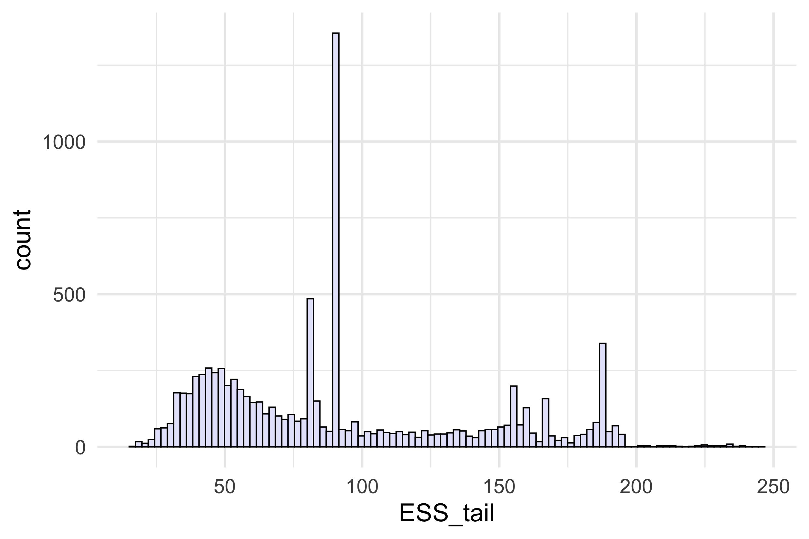
Effective sample size

Model assessment on simulated data

For the model assessment, we simulate data from the fitted model and plot the distribution of the median of protein expression.

# Simulated data
x_sim <- samples$x_sim # iteration * samples * ASVs
# Choose only the first chain
x_sim <- x_sim[1:(iter/2), ,] # For each iteration, simulated data is x_sim[i, ,]
x_med_asv <- apply(x %>% data.frame , 2, median)
sim_ite <- dim(x_sim)[1]
ite_plot <- 19# or ite_plot <- sim_ite
#Find maximum of each asv for each iteration
med_all <- data.frame(x_med_asv = x_med_asv)
for(i in 1:ite_plot){
  x_sim_i <- x_sim[i, ,]
  med_x_sim_i <- apply(x_sim_i %>% data.frame , 2, median)
  med_all <- cbind(med_all, med_x_sim_i)
}

colnames(med_all) <- c("x_med_asv", paste0("x_med_sim_1", seq(1, ite_plot)))
avg_med_square <- numeric()

# histogram of maximum
med_all_long <- melt(med_all)
med_all_long$type <- c(rep("observed", dim(x_sim)[3]), rep("simulated", dim(x_sim)[3]*(ite_plot)))
med_all_long$type <- factor(med_all_long$type)
p_hist_obs_sim <- ggplot(data = med_all_long) +
  geom_histogram(aes(x = value, group = variable, fill = type),
                 colour = "black",
                 bins = 100) +
  facet_wrap(~variable, nrow = 5) +
  theme(legend.position = "none")

p_hist_obs_sim
# ggsave(paste0("model_assesment_hist_obs_sim_mibi_cytof_one_K_",K, ".png"), p_hist_obs_sim, width = 12, height = 6)

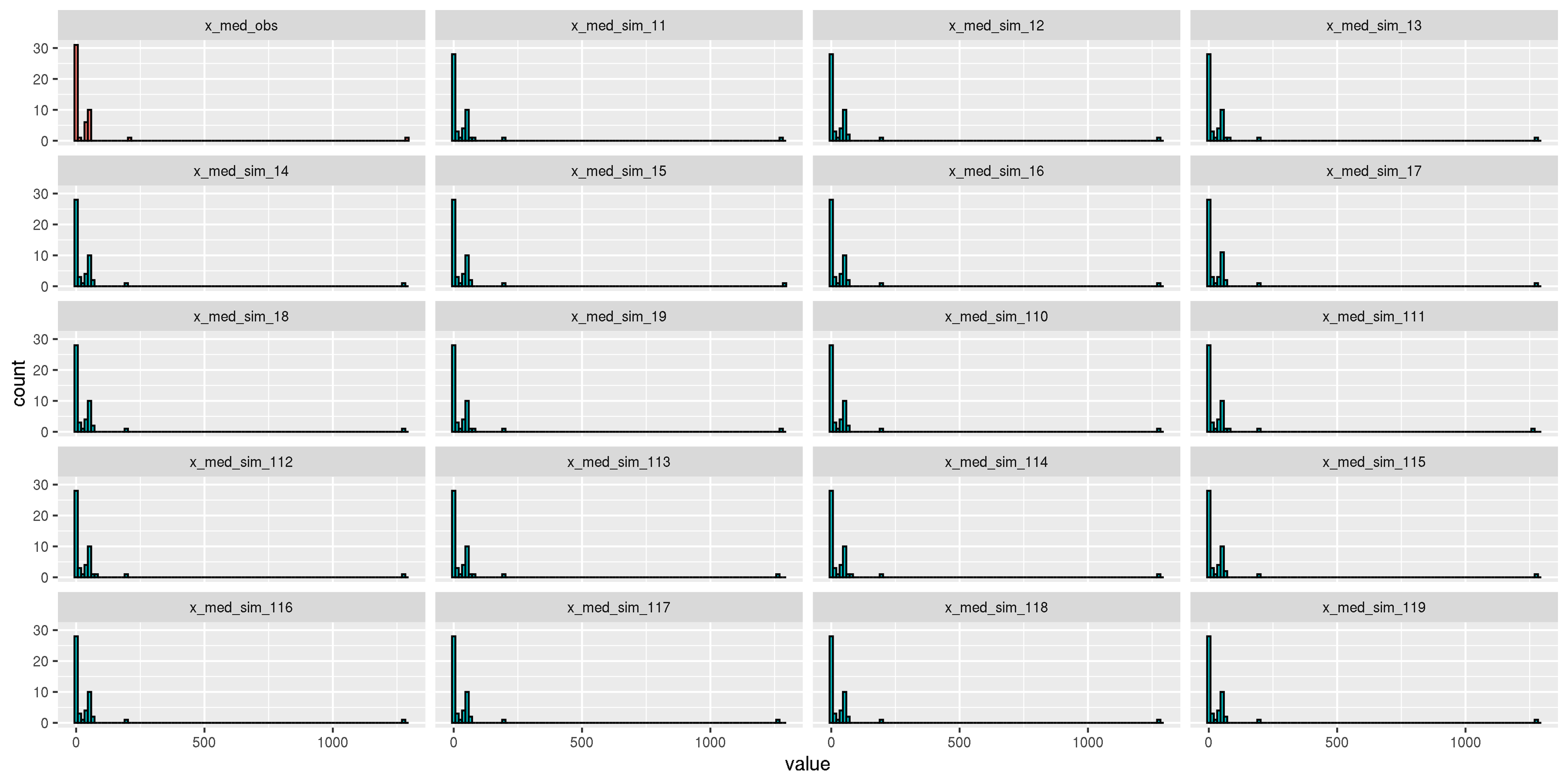
Model assessment.

The distribution of the observed median of each protein expression (first facet) is similar to the median of simulated data from the fitted topic model (other facets).

Infer spatial location of CyTOF immune cells

We use the sample from the first chain.

theta <- samples$theta
theta_aligned <- theta[1:(iter/2), ,]
dimnames(theta_aligned)[[2]] <- mae_train$cell_id
dimnames(theta_aligned)[[3]] <- c(paste0("Topic_", seq(1,K)))

# array to a dataframe
theta_all <- melt(theta_aligned)
colnames(theta_all) <- c("iteration", "Sample", "Topic", "topic.dis")
theta_all$Chain <- paste0("Chain ", rep(seq(1, 1), each = (iter/2)))

sam <- colData(mae_train) %>% data.frame()
theta_all$Sample <- as.character(theta_all$Sample)
theta_all <- left_join(theta_all, sam, by =c("Sample"= "cell_id"))
theta_all$Chain <- factor(theta_all$Chain)
theta_all$Topic <- factor(theta_all$Topic)
theta_all$Sample <- factor(theta_all$Sample)

theta_all$cell_type <- factor(theta_all$cell_type)
theta_all$method <- ifelse(is.na(theta_all$cell_type), "cytof", as.character(theta_all$cell_type))

Based on the median topic distribution, we identify the most dominant topic in each cell.

theta_summary <- theta_all %>%
  group_by(Sample, Topic, method) %>%
  summarize(median.topic.dis = median(topic.dis)) %>%
  ungroup() %>%
  mutate(Topic = factor(Topic, levels = rev(str_c("Topic_",1:K))))

theta_summary_2 <- theta_summary %>%
  dplyr::group_by(Sample) %>%
  dplyr::summarise(
    max_topic = max(median.topic.dis),
    Topic = Topic[which(median.topic.dis == max(median.topic.dis))],
    method = method[1]
  )

# saveRDS(theta_summary_2, paste0("../Results/co_location_mibi_cytof_one_K_", K, ".rds"))

theta_summary_2 <- readRDS(paste0("co_location_mibi_cytof_one_K_", K, ".rds"))

MIBI has only one site, so we may not infer spatial location for some cells in CyTOF.

# mibi X, Y coordinates
df <- data.frame(Sample = mae_train$cell_id, X = mae_train$centroid_X, Y = mae_train$centroid_Y)
df <- left_join(theta_summary_2, df, by = "Sample") %>% data.frame()
df$Sample <- as.character(df$Sample)
rownames(df) <- df$Sample
for(i in 1:dim(df)[1]){
  if(df$method[i] == "cytof"){
    #subset the df mibi cells with the topic for ith cytof cell
    df_i <- dplyr::filter(df, Topic == df$Topic[i] & method != "cytof")
    com_cell_close_to_max_topic_i <- df_i$Sample[which(abs(df$max_topic[i] - df_i$max_topic) == min(abs(df$max_topic[i] - df_i$max_topic)))]
    if(length(which(df$Sample == com_cell_close_to_max_topic_i))==0){
      df$X[i] <- NA
    }else{
      df$X[i] <- df$X[which(df$Sample == com_cell_close_to_max_topic_i)]
    }
    if(length(which(df$Sample == com_cell_close_to_max_topic_i)) == 0){
      df$Y[i] <- NA
    }else{
      df$Y[i] <- df$Y[which(df$Sample == com_cell_close_to_max_topic_i)]
    }

  }
}

Plot the spatial location of CyTOF cells from patient BB028.

manual_col <- tableau_color_pal("Classic 20")(length(unique(df$method)))
df$method <- factor(df$method)
df_cytof <- dplyr::filter(df, method == "cytof")
p_co <- ggplot(data = df) +
  geom_point(aes(x= X, y = Y, col = method), size = 5) +
  theme_minimal() +
  scale_color_manual(values = manual_col)  +
  theme(aspect.ratio = 1, legend.position = "right") +
  labs(fill = "method") +
  xlim(c(0, max(df$X))) +
  ylim(c(0, max(df$Y))) +
  geom_text(data = df_cytof, aes(x = X, y= Y, label = Sample), check_overlap = TRUE)

p_co

# ggsave(paste0("co_location_mibi_cytof_one_K_", K, ".png"), p_co, width = 15, height = 15)

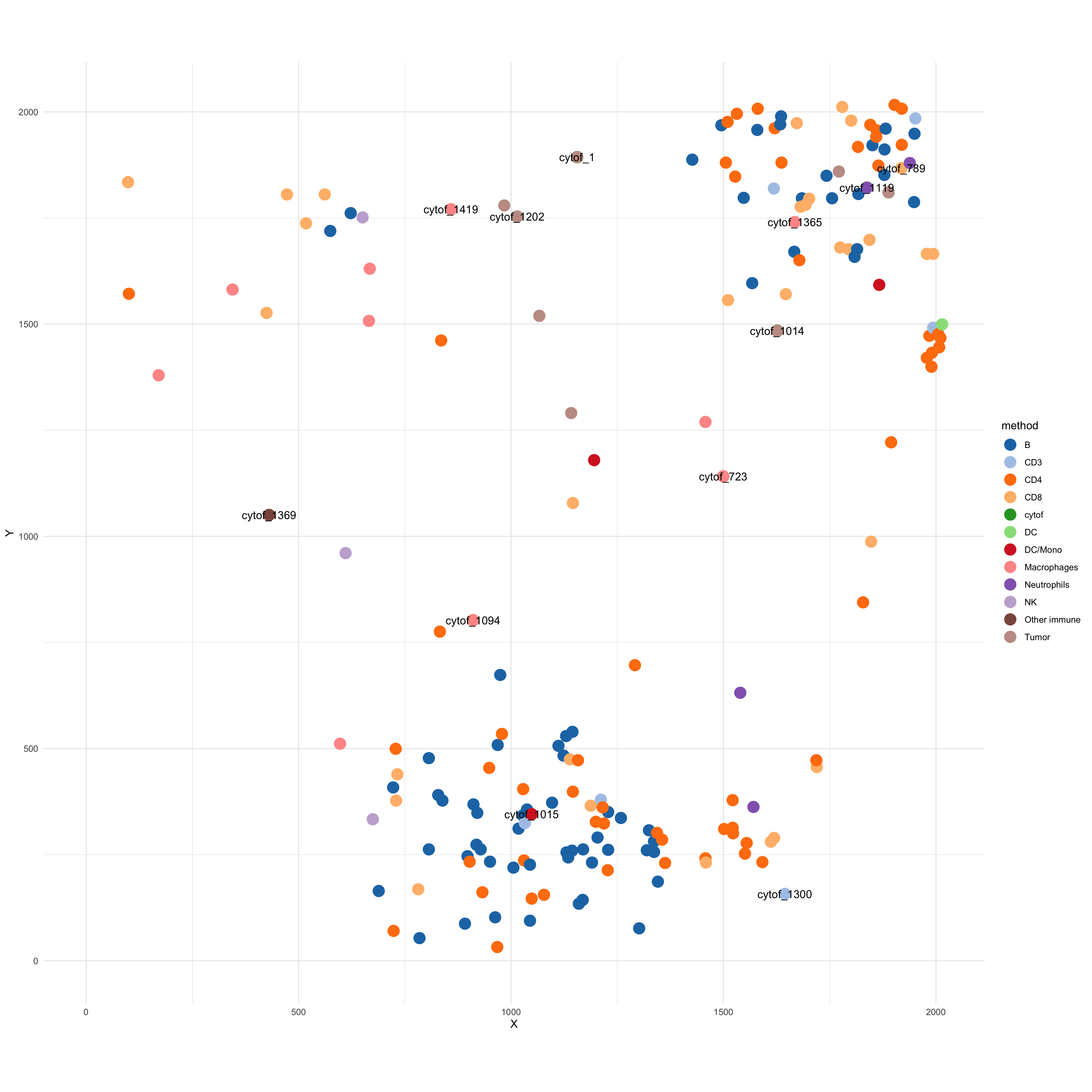
Labels show the inferred co-location of immune cells from CyTOF data (some are overlapping). We assign the spatial location of MIBI-TOF cells to the CyTOF data based on each cell’s topic distribution.

Predict spatial pattern of proteins not measured in the MIBI-TOF

proteins_not_measured_mibi <- rowData(mae[["cd45"]])$marker_name[!(as.character(rowData(mae[["cd45"]])$marker_name) %in% as.character(rowData(mae[["mibi"]])$channel_name))] %>% as.character()

# Simulated data
x_sim <- samples$x_sim # iteration * samples * ASVs
# Choose only the first chain
x_sim <- x_sim[1, ,] # For each iteration, simulated data 
colnames(x_sim) <- colnames(x_train)
rownames(x_train) <- rownames(x_train)
ind_mibi <- which(rownames(x_train) %in% colnames(assay(mae_train[["mibi"]])))
x_sim_mibi <- x_sim[ind_mibi, ]
ind_pro <- which(colnames(x_train) %in% proteins_not_measured_mibi)
ind_pro_present <- which(!(colnames(x_train) %in% proteins_not_measured_mibi))

x_sim_mibi_only_measured <- x_train[ind_mibi, ind_pro_present]
x_sim_mibi_only_measured_t <- asinh(x_sim_mibi_only_measured)

x_sim_mibi_predict <- x_sim_mibi
x_sim_mibi_predict_t <- asinh(x_sim_mibi_predict)


# UMAP of measured proteins
mibi_umap <- umap(x_sim_mibi_only_measured_t)
umap_df <- data.frame(UMAP1 = mibi_umap[,1],
                      UMAP2 = mibi_umap[,2],
                      cell_id = colData(mae_train)$cell_id[ind_mibi])
mibi_cell_data <- colData(mae_train)[ind_mibi, ] %>% data.frame()
umap_df  <- left_join(umap_df, mibi_cell_data, by = "cell_id")

manual_col <- tableau_color_pal("Classic 20")(length(unique(mae_train$cell_type)))

p1 <- ggplot(data = umap_df,
       aes(x = UMAP1, y = UMAP2, color = cell_type)) +
  geom_point(size = 3) +
  theme_bw() +
  scale_color_manual(values = manual_col)  +
  labs(color = "Cell types") +
  ggtitle("UMAP with measured proteins") +
  theme(aspect.ratio = 1, plot.title = element_text(hjust = 0.5))
p1

# Simulated data
x_sim <- samples$x_sim # iteration * samples * ASVs
# Choose only the first chain
x_sim <- x_sim[4, ,] # For each iteration, simulated data 
colnames(x_sim) <- colnames(x_train)
rownames(x_train) <- rownames(x_train)
ind_mibi <- which(rownames(x_train) %in% colnames(assay(mae_train[["mibi"]])))
x_sim_mibi <- x_sim[ind_mibi, ]
ind_pro <- which(colnames(x_train) %in% proteins_not_measured_mibi)
ind_pro_present <- which(!(colnames(x_train) %in% proteins_not_measured_mibi))

x_sim_mibi_only_measured <- x_train[ind_mibi, ind_pro_present]
x_sim_mibi_only_measured_t <- asinh(x_sim_mibi_only_measured)

x_sim_mibi_predict <- x_sim_mibi
x_sim_mibi_predict_t <- asinh(x_sim_mibi_predict)


manual_col <- tableau_color_pal("Classic 20")(length(unique(mae_train$cell_type)))


# UMAP of measured and predicted protein expression
mibi_umap <- umap(x_sim_mibi_predict_t)
umap_df <- data.frame(UMAP1 = mibi_umap[,1],
                      UMAP2 = mibi_umap[,2],
                      cell_id = colData(mae_train)$cell_id[ind_mibi])
mibi_cell_data <- colData(mae_train)[ind_mibi, ] %>% data.frame()
umap_df  <- left_join(umap_df, mibi_cell_data, by = "cell_id")

manual_col <- tableau_color_pal("Classic 20")(length(unique(mae_train$cell_type)))

p22 <- ggplot(data = umap_df,
       aes(x = UMAP1, y = UMAP2, color = cell_type)) +
  geom_point(size = 3) +
  theme_bw() +
  scale_color_manual(values = manual_col) +
  labs(color = "Cell types") +
  ggtitle("UMAP with measured and predicted proteins") +
  theme(aspect.ratio = 1, plot.title = element_text(hjust = 0.5))
p22

# Simulated data
x_sim <- samples$x_sim # iteration * samples * ASVs
# Choose only the first chain
x_sim <- x_sim[2, ,] # For each iteration, simulated data 
colnames(x_sim) <- colnames(x_train)
rownames(x_train) <- rownames(x_train)
ind_mibi <- which(rownames(x_train) %in% colnames(assay(mae_train[["mibi"]])))
x_sim_mibi <- x_sim[ind_mibi, ]
ind_pro <- which(colnames(x_train) %in% proteins_not_measured_mibi)
ind_pro_present <- which(!(colnames(x_train) %in% proteins_not_measured_mibi))

x_sim_mibi_only_measured <- x_train[ind_mibi, ind_pro_present]
x_sim_mibi_only_measured_t <- asinh(x_sim_mibi_only_measured)

x_sim_mibi_predict <- x_sim_mibi
x_sim_mibi_predict_t <- asinh(x_sim_mibi_predict)



manual_col <- tableau_color_pal("Classic 20")(length(unique(mae_train$cell_type)))


# UMAP of measured and predicted protein
# UMAP of measured proteins
mibi_umap <- umap(x_sim_mibi_predict_t)
umap_df <- data.frame(UMAP1 = mibi_umap[,1],
                      UMAP2 = mibi_umap[,2],
                      cell_id = colData(mae_train)$cell_id[ind_mibi])
mibi_cell_data <- colData(mae_train)[ind_mibi, ] %>% data.frame()
umap_df  <- left_join(umap_df, mibi_cell_data, by = "cell_id")

manual_col <- tableau_color_pal("Classic 20")(length(unique(mae_train$cell_type)))

p23 <- ggplot(data = umap_df,
       aes(x = UMAP1, y = UMAP2, color = cell_type)) +
  geom_point(size = 3) +
  theme_bw() +
  scale_color_manual(values = manual_col) +
  labs(color = "Cell types")+
  ggtitle("UMAP with measured and predicted proteins") +
  theme(aspect.ratio = 1, plot.title = element_text(hjust = 0.5))
p23

com_p <- grid.arrange(p1, arrangeGrob(p22, p23, ncol=1), ncol=2, widths=c(1,1.2))

# ggsave("predicted_mibi_protein.png", com_p, width = 20, height = 15)

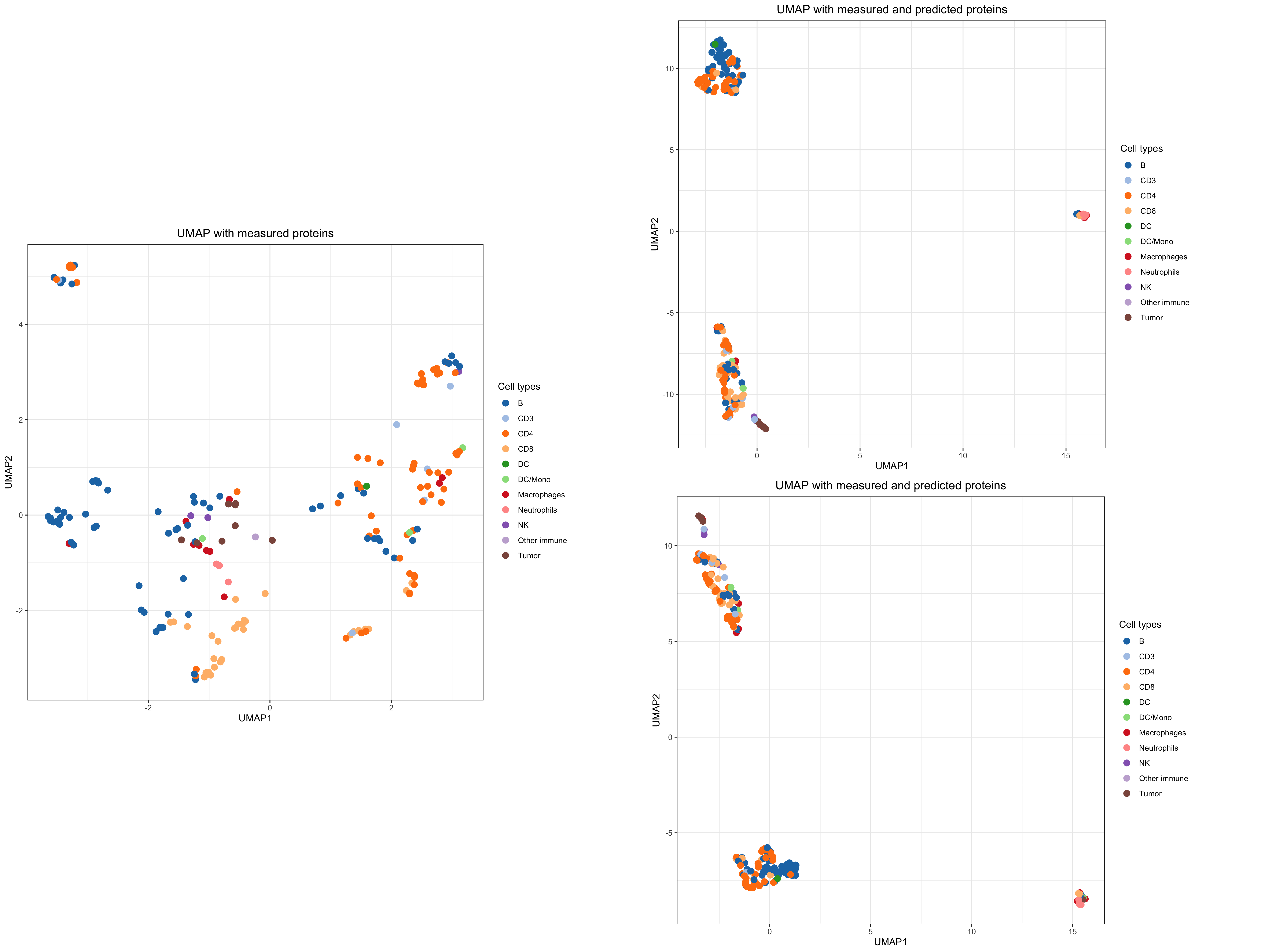
On the left, the first two dimensions of UMAP on the observed markers in the MIBI-TOF data. On the right, the first two dimensions of UMAP on the simulated data from the fitted model with predicted marker expression were not observed in MIBI-TOF data.

The clusters of cells are identified when using observed and predicted protein expressions.

References

Blei, David M, Andrew Y Ng, and Michael I Jordan. 2003. “Latent Dirichlet Allocation.” Journal of Machine Learning Research 3 (Jan): 993–1022.

Hastie, Trevor, Robert Tibshirani, Balasubramanian Narasimhan, and Gilbert Chu. 2019. Impute: Impute: Imputation for Microarray Data.

Keren, Leeat, Marc Bosse, Diana Marquez, Roshan Angoshtari, Samir Jain, Sushama Varma, Soo-Ryum Yang, et al. 2018. “A Structured Tumor-Immune Microenvironment in Triple Negative Breast Cancer Revealed by Multiplexed Ion Beam Imaging.” Cell 174 (6). Elsevier: 1373–87.

Ramos, Marcel, Lucas Schiffer, Angela Re, Rimsha Azhar, Azfar Basunia, Carmen Rodriguez, Tiffany Chan, et al. 2017. “Software for the Integration of Multiomics Experiments in Bioconductor.” Cancer Research 77 (21). AACR: e39–e42.

Wagner, Johanna, Maria Anna Rapsomaniki, Stéphane Chevrier, Tobias Anzeneder, Claus Langwieder, August Dykgers, Martin Rees, et al. 2019. “A Single-Cell Atlas of the Tumor and Immune Ecosystem of Human Breast Cancer.” Cell 177 (5). Elsevier: 1330–45.

jpratheepa31@gmail.com ↩

Latent Dirichlet Allocation to Integrate Single-Cell Targeted Proteomics Data

Prathee Jeganathan¹

Introduction

Method

Results

Subject selection

Data

Mass-Tag CyTOF Breast Cancer Data

Keren et al., MIBI-TOF Breast Cancer Data

Spatial information

Multiplicative error due to different scales

Converting each scale to have the same lower and upper levels

Merge two `SingleCellExperiment` objects and make `MultiAssayExperiment`

Join the assays and impute

Topic modeling

Split train and test set

Input for topic model

Visualization

Extract posterior samples

Alignment

Feature distribution

Computing statistics after alignment

Log posterior on the test data

Convergence diagnostics

Model assessment on simulated data

Infer spatial location of CyTOF immune cells

Predict spatial pattern of proteins not measured in the MIBI-TOF

References

Latent Dirichlet Allocation to Integrate Single-Cell Targeted Proteomics Data

Prathee Jeganathan1

Introduction

Method

Results

Subject selection

Data

Mass-Tag CyTOF Breast Cancer Data

Keren et al., MIBI-TOF Breast Cancer Data

Spatial information

Multiplicative error due to different scales

Converting each scale to have the same lower and upper levels

Merge two SingleCellExperiment objects and make MultiAssayExperiment

Join the assays and impute

Topic modeling

Split train and test set

Input for topic model

Visualization

Extract posterior samples

Alignment

Feature distribution

Computing statistics after alignment

Log posterior on the test data

Convergence diagnostics

Model assessment on simulated data

Infer spatial location of CyTOF immune cells

Predict spatial pattern of proteins not measured in the MIBI-TOF

References

Prathee Jeganathan¹

Merge two `SingleCellExperiment` objects and make `MultiAssayExperiment`